Chapter 15. Demand Management and Forecasting

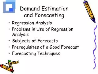
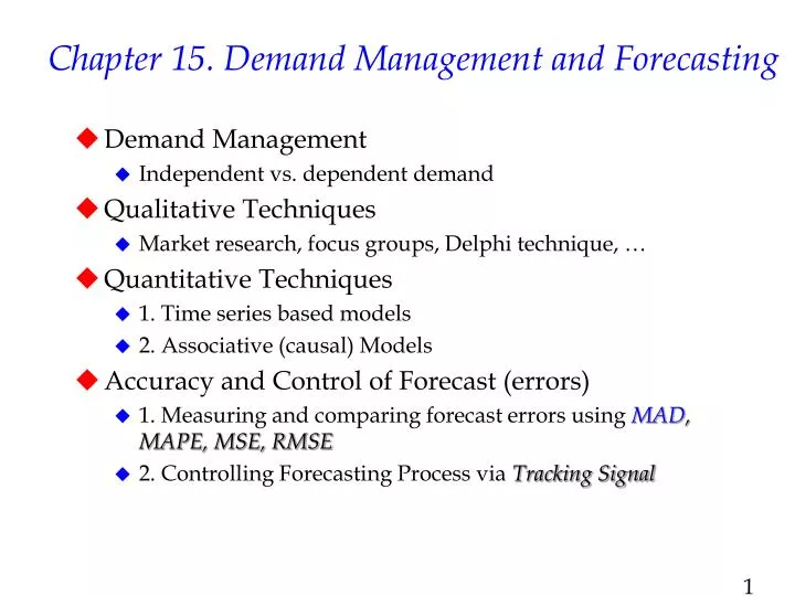
1. Chapter 15. Demand Management and Forecasting • Demand Management • Independent vs. dependent demand • Qualitative Techniques • Market research, focus groups, Delphi technique, … • Quantitative Techniques • 1. Time series based models • 2. Associative (causal) Models • Accuracy and Control of Forecast (errors) • 1. Measuring and comparing forecast errors using MAD, MAPE, MSE, RMSE • 2. Controlling Forecasting Process via Tracking Signal

2. Independent Demand: Finished Goods Dependent Demand: Raw Materials, Component parts, Sub-assemblies, etc. C(2) B(4) D(2) E(1) D(3) F(2) Demand Management A

3. Demand Management • Active role to influence demand. • Examples from seasonal goods or services • Campaigns, discounts, etc. • Incentives to sales personnel • Passive role, limited or no action taken. • Why?

4. Qualitative Methods Market Research Grass Roots Qualitative Methods Panel Consensus Historical analogy Executive Judgment Delphi Method

5. Delphi Method • Choose the experts to participate representing a variety of knowledgeable people in different areas • Through a questionnaire (or E-mail), obtain forecasts (and any premises or qualifications for the forecasts) from all participants • Summarize the results and redistribute them to the participants along with appropriate new questions • Summarize again, refining forecasts and conditions, and again develop new questions • Repeat Step 4 as necessary and distribute the final results to all participants

6. Time series models Past predicts future Uses time series data Key variable: time (t) Easier to apply Less accurate Examples: Moving averages Exponential smoothing Causal models Examines potential cause=> effect relationships Requires cross sectional data Key variables are usually denoted as X1 , X2 , X3 , … More difficult Takes more time But worth it since it provides insight to the system (process) under study Examples: Various regression models Quantitative forecasting methods

7. Quantitative techniques • Basic time series approaches • i. Moving averages, simple &weighted • ii. Exponential smoothing, simple & trend adjusted • iii. Linear regression (linear trend model) • iv. Techniques for seasonality and trend - Decomposition of time series • Causal approach • i. Simple Linear Regression • ii. Multiple Linear Regression

8. 15-8 Seasonal variation x x x x x x x x x x x x x x x x x x x x x x x x x x x x x x x x x x x x x x x x x x x x x x x 1 2 3 4 Year Finding Components of a Time Series Linear Trend Sales

9. What to look for in a time series • Trend - long-term movement in data • Seasonality - short-term regular and repetitive variations in data • Cyclical variations – long(er) term, occasionally caused by unusual circumstances, (war, economic downturn, etc.) • Autocorrelation – denotes persistence of occurrence (momentum driven) • Random variations - caused by chance

10. Moving Averages • Simple moving average (MA) • Ft = Forecast for the coming period • n = Number of periods to be averaged • A t-1 = Actual occurrence in the past period for up to “n” periods • Weighted moving average (WMA) permits an unequal weighting on prior time periods • Excel time! • Problem 20.

11. Exponential Smoothing Models • Simple exponential smoothing model • Alpha is the smoothing constant • Whenever appropriate more weight can be given to the more recent data (time periods) • Double exponential smoothing (Holt’s model) • Adds trend component, T and delta (gamma) as the smoothing constant for trend • Forecast Including Trend (FIT)  • Excel time! • Problem 20, continued.

12. Measuring Accuracy, Forecast Errors • To compare different time series techniques or to select the “best” set of initial values for the parameters, use a combination of the the following four metrics: • Mean Absolute Deviation • Most popular but • Mean Absolut Percent Error • Should be used in tandem with MAD • Mean Square Error • Root Mean Square Error

13. Tracking Signal • The Tracking Signal or TS is a measure that indicates whether the forecast average is keeping pace with any genuine upward or downward changes in demand. • Depending on the number of MAD’s selected, the TS can be used like a quality control chart indicating when the model is generating too much error in its forecasts. • TS is a monitoring system. • The TS formula is:

14. Regression analysis • Identify factors (independent variables) that can be used to predict the values for the forecast variable (e.g., sales). • Regression applied to “causal” data requires different kinds of data • Regression applied to “time series” data is also know as “trend line analysis” • We will use Excel (Tools/Data analysis) to obtain the regression line and all relevant statistics.

15. A simple regression example • The first example applies regression to “time series” data. • Whenever possible, plot and observe the data. • The scatter plot shows a linear relation between advertising and sales. So the following regression model is suggested by the data, which refers to the true relationship between the entire population of advertising and sales values. • Other common formats are:

16. Decomposition of a Time Series • Demand has both trend and seasonal components. • View data via Excel. • Compute overall average • Compute average of the same seasons of each cycle (e.g., year) • Compute seasonal indexes (seasonal averages / overall avg.) • Deseasonalize data (actual values /seasonal indexes) • Apply regression to deseasonalized data • Compute (project) deseasonalized forecasts using the regression equation • Reseasonalize the forecasts by multiplying them with the seasonal indexes. • Excel time. • Problem 21.

17. Multiple regression • Most regression problems involve more than one independent variable. • If each independent variables varies in a linear manner with Y, the estimated regression function in this case is: • Where b0 is the intercept (also called constant) • The optimal values for the bi(slopes) can again be found using the least squares method

18. Steps in multiple regression analysis • Hypotheses for testing whether a general linear model is useful is predicting Y: • Ho : ß1 = ß2 = ß3 = ... = ßk = 0 (means there is NOTHING useful) • HA : At least one of the ß parameters in Ho is nonzero. • Test statistic: F-statistic = MSR / MSE • If the model is deemed adequate (passes the F-test; rejected H0 ) then go to step 4(otherwise, none of variables have any impact on Y ) • Conduct t-tests (significance tests) on ß parameters (slopes). • Remove the most insignificantindependentvariable, re-run the regression, and go to step 4. • Repeat steps 4 & 5 until all remaining independent variable parameters (slopes) are significant, then go to step 7 • If the intercept (ß0 ) is insignificant then remove it, run regression one more time. • Excel time!

19. What Forecasters Should Do • Determine what elements of historical data provide repeatable patterns and utilize this to make extrapolations. • Make a list of the possible independent variables that may have influenced the historical data and may influence future outcomes. • Statistically correlate the independent variables to the outcome history using regression analysis to validate their importance and to calibrate their effects. • Make estimates of forecast error wherever possible using MAD or standard deviation measures. • Make clear presentations of the results and assumptions and listen to feedback.

20. Forecasting • Always remember that you (managers) are decision makers and sound decisions are based on good forecasts • Suggested problems: • 2, 3, 4, 7, 11, 12, 14, 17, 20, 21, 27