Download
1 / 66
740 likes | 1.2k Views
MIT Center for Materials Science and Engineering. Estimating Crystallite Size Using XRD. Scott A Speakman, Ph.D. 13-4009A speakman@mit.edu http://prism.mit.edu/xray. Warning. These slides have not been extensively proof-read, and therefore may contain errors.

E N D
MIT Center for Materials Science and Engineering Estimating Crystallite SizeUsing XRD Scott A Speakman, Ph.D. 13-4009A speakman@mit.edu http://prism.mit.edu/xray
Warning • These slides have not been extensively proof-read, and therefore may contain errors. • While I have tried to cite all references, I may have missed some– these slides were prepared for an informal lecture and not for publication. • If you note a mistake or a missing citation, please let me know and I will correct it. • I hope to add commentary in the notes section of these slides, offering additional details. However, these notes are incomplete so far. http://prism.mit.edu/xray
Goals of Today’s Lecture • Provide a quick overview of the theory behind peak profile analysis • Discuss practical considerations for analysis • Briefly mention other peak profile analysis methods • Warren Averbach Variance method • Mixed peak profiling • whole pattern • Discuss other ways to evaluate crystallite size • Assumptions: you understand the basics of crystallography, X-ray diffraction, and the operation of a Bragg-Brentano diffractometer http://prism.mit.edu/xray
A Brief History of XRD • 1895- Röntgen publishes the discovery of X-rays • 1912- Laue observes diffraction of X-rays from a crystal • 1913- Bragg solves the first crystal structure from X-ray diffraction data • when did Scherrer use X-rays to estimate the crystallite size of nanophase materials? http://prism.mit.edu/xray
The Scherrer Equation was published in 1918 • Peak width (B) is inversely proportional to crystallite size (L) • P. Scherrer, “Bestimmung der Grösse und der inneren Struktur von Kolloidteilchen mittels Röntgenstrahlen,” Nachr. Ges. Wiss. Göttingen26 (1918) pp 98-100. • J.I. Langford and A.J.C. Wilson, “Scherrer after Sixty Years: A Survey and Some New Results in the Determination of Crystallite Size,” J. Appl. Cryst.11 (1978) pp 102-113. http://prism.mit.edu/xray
X-Ray Peak Broadening is caused by deviation from the ideal crystalline lattice • The Laue Equations describe the intensity of a diffracted peak from an ideal parallelopipeden crystal • The ideal crystal is an infinitely large and perfectly ordered crystalline array • From the perspective of X-rays, “infinitely” large is a few microns • Deviations from the ideal create peak broadening • A nanocrystallite is not “infinitely” large • Non-perfect ordering of the crystalline array can include • Defects • Non-uniform interplanar spacing • disorder http://prism.mit.edu/xray
As predicted by the Laue equations, the diffraction peaks becomes broader when N is not infinite • N1, N2, and N3 are the number of unit cells along the a1, a2, and a3 directions • The calculated peak is narrow when N is a large number (ie infinitely large) • When N is small, the diffraction peaks become broader • A nanocrystallinephase has a small number of N • The peak area remains constant independent of N http://prism.mit.edu/xray
Intensity (a.u.) 66 67 68 69 70 71 72 73 74 2 q (deg.) We cannot assume that all broad peaks are produced by nanocrystalline materials • These diffraction patterns were produced from the exact same sample • Two different diffractometers, with different optical configurations, were used • The apparent peak broadening is due solely to the instrumentation http://prism.mit.edu/xray
Many factors may contribute tothe observed peak profile • Instrumental Peak Profile • Crystallite Size • Microstrain • Non-uniform Lattice Distortions • Faulting • Dislocations • Antiphase Domain Boundaries • Grain Surface Relaxation • Solid Solution Inhomogeneity • Temperature Factors • The peak profile is a convolution of the profiles from all of these contributions http://prism.mit.edu/xray
Intensity (a.u.) 46.7 46.8 46.9 47.0 47.1 47.2 47.3 47.4 47.5 47.6 47.7 47.8 47.9 2 q (deg.) Intensity (a.u.) 46.7 46.8 46.9 47.0 47.1 47.2 47.3 47.4 47.5 47.6 47.7 47.8 47.9 2 q (deg.) Before analysis, you must decide how you will define Peak Width • Full Width at Half Maximum (FWHM) • the width of the diffraction peak, in radians, at a height half-way between background and the peak maximum • This was most often used in older research because it is easier to calculate • Integral Breadth • the total area under the peak divided by the peak height • the width of a rectangle having the same area and the same height as the peak • requires very careful evaluation of the tails of the peak and the background FWHM http://prism.mit.edu/xray
Integral Breadth may be the way to define peak width with modern analysis software • Warren suggests that the Stokes and Wilson method of using integral breadths gives an evaluation that is independent of the distribution in size and shape • L is a volume average of the crystal thickness in the direction normal to the reflecting planes • The Scherrer constant K can be assumed to be 1 • Langford and Wilson suggest that even when using the integral breadth, there is a Scherrer constant K that varies with the shape of the crystallites http://prism.mit.edu/xray
Other methods used to determine peak width • These methods are used in more the variance methods, such as Warren-Averbach analysis • Most often used for dislocation and defect density analysis of metals • Can also be used to determine the crystallite size distribution • Requires no overlap between neighboring diffraction peaks • Variance-slope • the slope of the variance of the line profile as a function of the range of integration • Variance-intercept • negative initial slope of the Fourier transform of the normalized line profile http://prism.mit.edu/xray
Instrument and Sample Contributions to the Peak Profile must be Deconvoluted • In order to analyze crystallite size, we must deconvolute: • Instrumental Broadening FW(I) • also referred to as the Instrumental Profile, Instrumental FWHM Curve, Instrumental Peak Profile • Specimen Broadening FW(S) • also referred to as the Sample Profile, Specimen Profile • We must then separate the different contributions to specimen broadening • Crystallite size and microstrain broadening of diffraction peaks • This requires an Instrument Profile Calibration Curve http://prism.mit.edu/xray
Intensity (a.u.) 47.0 47.2 47.4 47.6 47.8 2 q (deg.) The Instrument Peak Profile Calibration Curve quantifies the contribution of the instrument to the observed peak widths • The peak widths from the instrument peak profile are a convolution of: • X-ray Source Profile • Wavelength widths of Ka1 and Ka2 lines • Size of the X-ray source • Superposition of Ka1 and Ka2 peaks • Goniometer Optics • Divergence and Receiving Slit widths • Imperfect focusing • Beam size • Penetration into the sample Patterns collected from the same sample with different instruments and configurations at MIT http://prism.mit.edu/xray
Other Instrumental and Sample Considerations for Thin Films • The irradiated area greatly affects the intensity of high angle diffraction peaks • GIXD or variable divergence slits on the PANalyticalX’Pert Pro will maintain a constant irradiated area, increasing the signal for high angle diffraction peaks • both methods increase the instrumental FWHM • Bragg-Brentano geometry only probes crystallite dimensions through the thickness of the film • in order to probe lateral (in-plane) crystallite sizes, need to collect diffraction patterns at different tilts • this requires the use of parallel-beam optics on the PANalyticalX’Pert Pro, which have very large FWHM and poor signal:noise ratios http://prism.mit.edu/xray
In order to build a Instrument Peak Profile Calibration Curve • Collect data from a standard using the exact instrument and configuration as will be used for analyzing the sample • same optical configuration of diffractometer • same sample preparation geometry • You need a separate calibration curve for every different instrument and instrument configuration • Even a small change, such as changing the divergence slit from ½ to ¼° aperture, will change the instrument profile • calibration curve should cover the 2theta range of interest for the specimen diffraction pattern • do not extrapolate the calibration curve • Profile fit the diffraction peaks from the standard • Fit the peak widths to a function such as the Cagliotti equation. Use this function as the calibration curve. http://prism.mit.edu/xray
The Cagliotti equation describes how peak width varies with 2theta • Hk is the Cagliotti function where U, V and W are refinable parameters
Selecting a standard for building the Instrument Peak Profile Calibration Curve • Standard should share characteristics with the nanocrystalline specimen • Similar linear absorption coefficient • similar mass absorption coefficient • similar atomic weight • similar packing density • The standard should not contribute to the diffraction peak profile • macrocrystalline: crystallite size larger than 500 nm • particle size less than 10 microns • defect and strain free • There are several calibration techniques • Internal Standard • External Standard of same composition • External Standard of different composition http://prism.mit.edu/xray
Internal Standard Method for Calibration • Mix a standard in with your nanocrystalline specimen • a NIST certified standard is preferred • use a standard with similar mass absorption coefficient • NIST 640c Si • NIST 660a LaB6 • NIST 674b CeO2 • NIST 675 Mica • standard should have few, and preferably no, overlapping peaks with the specimen • overlapping peaks will greatly compromise accuracy of analysis http://prism.mit.edu/xray
Internal Standard Method for Calibration • Advantages: • know that standard and specimen patterns were collected under identical circumstances for both instrumental conditions and sample preparation conditions • the linear absorption coefficient of the mixture is the same for standard and specimen • Disadvantages: • difficult to avoid overlapping peaks between standard and broadened peaks from very nanocrystalline materials • the specimen becomes contaminated • only works with a powder specimen http://prism.mit.edu/xray
External Standard Method for Calibration • If internal calibration is not an option, then use external calibration • Run calibration standard separately from specimen, keeping as many parameters identical as is possible • The best external standard is a macrocrystalline specimen of the same phase as your nanocrystalline specimen • How can you be sure that macrocrystalline specimen does not contribute to peak broadening? http://prism.mit.edu/xray
Qualifying your Macrocrystalline Standard • select powder for your potential macrocrystalline standard • if not already done, possibly anneal it to allow crystallites to grow and to allow defects to heal • use internal calibration to validate that macrocrystalline specimen is an appropriate standard • mix macrocrystalline standard with appropriate NIST SRM • compare FWHM curves for macrocrystalline specimen and NIST standard • if the macrocrystalline FWHM curve is similar to that from the NIST standard, than the macrocrystalline specimen is suitable • collect the XRD pattern from pure sample of you macrocrystalline specimen • do not use the FHWM curve from the mixture with the NIST SRM http://prism.mit.edu/xray
Disadvantages/Advantages of External Calibration with a Standard of the Same Composition • Advantages: • will produce better calibration curve because mass absorption coefficient, density, molecular weight are the same as your specimen of interest • can duplicate a mixture in your nanocrystalline specimen • might be able to make a macrocrystalline standard for thin film samples • Disadvantages: • time consuming • desire a different calibration standard for every different nanocrystalline phase and mixture • macrocrystalline standard may be hard/impossible to produce • calibration curve will not compensate for discrepancies in instrumental conditions or sample preparation conditions between the standard and the specimen http://prism.mit.edu/xray
External Standard Method of Calibration using a NIST standard • As a last resort, use an external standard of a composition that is different than your nanocrystalline specimen • This is actually the most common method used • Also the least accurate method • Use a certified NIST standard to produce instrumental FWHM calibration curve • Use the standard that has the most similar linear absorption coefficient http://prism.mit.edu/xray
Advantages and Disadvantages of using NIST standard for External Calibration • Advantages • only need to build one calibration curve for each instrumental configuration • I have NIST standard diffraction patterns for each instrument and configuration available for download from http://prism.mit.edu/xray/standards.htm • know that the standard is high quality if from NIST • neither standard nor specimen are contaminated • Disadvantages • The standard may behave significantly different in diffractometer than your specimen • different mass absorption coefficient • different depth of penetration of X-rays • NIST standards are expensive • cannot duplicate exact conditions for thin films http://prism.mit.edu/xray
Consider- when is good calibration most essential? Broadening Due to Nanocrystalline Size • For a very small crystallite size, the specimen broadening dominates over instrumental broadening • Only need the most exacting calibration when the specimen broadening is small because the specimen is not highly nanocrystalline FWHM of Instrumental Profile at 48° 2q 0.061 deg http://prism.mit.edu/xray
What Instrument to Use? • The instrumental profile determines the upper limit of crystallite size that can be evaluated • if the Instrumental peak width is much larger than the broadening due to crystallite size, then we cannot accurately determine crystallite size • For analyzing larger nanocrystallites, it is important to use the instrument with the smallest instrumental peak width • Very small nanocrystallites produce weak signals • the specimen broadening will be significantly larger than the instrumental broadening • the signal:noise ratio is more important than the instrumental profile http://prism.mit.edu/xray
Comparison of Peak Widths at 47° 2q for Instruments and Crystallite Sizes • Instruments with better peak height to background ratios are better for small nanocrystallites, <20nm • Instruments with smaller instrumental peak widths are better for larger nanocrystallites, >80 nm http://prism.mit.edu/xray
For line profile analysis, must remove the instrument contribution to each peak list • When analyzing the diffraction pattern from the sample, the instrument contribution to the peak width must be removed • The instrument contribution is convoluted with the specimen contribution to peak broadening • Peak deconvolution is a difficult process, so simpler calculations are often used • Most commonly, the observed peak width is treated as the sum of the instrument and specimen contributions • This works well when: • crystallite size is the dominant contribution to peak broadening • The peak broadening is largely Lorentzian in shape • Other analysis will treat the observed peak as the sum of the squares of the instrument and specimen contributions • This works well when: • microstrain is the dominant contribution to peak broadening • The peak broadening is largely Gaussian in shape http://prism.mit.edu/xray
Once the instrument broadening contribution has been remove, the specimen broadening can be analyzed • Contributions to specimen broadening • Crystallite Size • Microstrain • Non-uniform Lattice Distortions • Faulting • Dislocations • Antiphase Domain Boundaries • Grain Surface Relaxation • Solid Solution Inhomogeneity • Temperature Factors • The peak profile is a convolution of the profiles from all of these contributions http://prism.mit.edu/xray
Crystallite Size Broadening • Peak Width due to crystallite size varies inversely with crystallite size • as the crystallite size gets smaller, the peak gets broader • The peak width varies with 2q as cos q • The crystallite size broadening is most pronounced at large angles 2Theta • However, the instrumental profile width and microstrain broadening are also largest at large angles 2theta • peak intensity is usually weakest at larger angles 2theta • If using a single peak, often get better results from using diffraction peaks between 30 and 50 deg 2theta • below 30deg 2theta, peak asymmetry compromises profile analysis http://prism.mit.edu/xray
The Scherrer Constant, K • The constant of proportionality, K (the Scherrer constant) depends on the how the width is determined, the shape of the crystal, and the size distribution • K actually varies from 0.62 to 2.08 • the most common values for K are: • 0.94 for FWHM of spherical crystals with cubic symmetry • 0.89 for integral breadth of spherical crystals w/ cubic symmetry • 1, because 0.94 and 0.89 both round up to 1 • For an excellent discussion of K, refer to JI Langford and AJC Wilson, “Scherrer after sixty years: A survey and some new results in the determination of crystallite size,” J. Appl. Cryst.11 (1978) p102-113. http://prism.mit.edu/xray
Factors that affect K and crystallite size analysis • how the peak width is defined • Whether using FWHM or Integral Breadth • Integral breadth is preferred • how crystallite size is defined • the shape of the crystal • the size distribution http://prism.mit.edu/xray
How is Crystallite Size Defined • Usually taken as the cube root of the volume of a crystallite • assumes that all crystallites have the same size and shape • None of the X-ray diffraction techniques give a crystallite size that exactly matches this definition • For a distribution of sizes, the mean size can be defined as • the mean value of the cube roots of the individual crystallite volumes • the cube root of the mean value of the volumes of the individual crystallites • Scherrer method (using FWHM) gives the ratio of the root-mean-fourth-power to the root-mean-square value of the thickness • Stokes and Wilson method (using integral breadth) determines the volume average of the thickness of the crystallites measured perpendicular to the reflecting plane • The variance methods give the ratio of the total volume of the crystallites to the total area of their projection on a plane parallel to the reflecting planes http://prism.mit.edu/xray
The Stokes and Wilson method considers that each different diffraction peak is produced from planes along a different crystallographic direction • Stokes and Wilson method (using integral breadth) determines the volume average of the thickness of the crystallites measured perpendicular to the reflecting plane • This method is useful for identifying anisotropic crystallite shapes (002) a-axis // [200] c-axis, // [002] (200) http://prism.mit.edu/xray
Remember, Crystallite Size is Different than Particle Size • A particle may be made up of several different crystallites • Crystallite size often matches grain size, but there are exceptions http://prism.mit.edu/xray
The crystallite size observed by XRD is the smallest undistorted region in a crystal • Dislocations may create small-angle domain boundaries • Dipolar dislocation walls will also create domain boundaries http://prism.mit.edu/xray
Crystallite Shape • Though the shape of crystallites is usually irregular, we can often approximate them as: • sphere, cube, tetrahedra, or octahedra • parallelepipeds such as needles or plates • prisms or cylinders • Most applications of Scherrer analysis assume spherical crystallite shapes • If we know the average crystallite shape from another analysis, we can select the proper value for the Scherrer constant K • Anistropic peak shapes can be identified by anistropic peak broadening • if the dimensions of a crystallite are 2x * 2y * 200z, then (h00) and (0k0) peaks will be more broadened then (00l) peaks. http://prism.mit.edu/xray
Anistropic Size Broadening • The broadening of a single diffraction peak is the product of the crystallite dimensions in the direction perpendicular to the planes that produced the diffraction peak. http://prism.mit.edu/xray
Crystallite Size Distribution • is the crystallite size narrowly or broadly distributed? • is the crystallite size unimodal? • XRD is poorly designed to facilitate the analysis of crystallites with a broad or multimodal size distribution • Variance methods, such as Warren-Averbach, can be used to quantify a unimodal size distribution • Otherwise, we try to accommodate the size distribution in the Scherrer constant • Using integral breadth instead of FWHM may reduce the effect of crystallite size distribution on the Scherrer constant K and therefore the crystallite size analysis http://prism.mit.edu/xray
Values for K referenced in HighScore Plus • Values of K from Langford and Wilson, J. Appl. Cryst (1978) are: • 0.94 for FWHM of spherical crystals with cubic symmetry • 0.89 for integral breadth of spherical crystals w/ cubic symmetry • 1, because 0.94 and 0.89 both round up to 1 • Assuming the Scherrer definition of crystallite size, values of K listed in the Help for HighScore Plus are: http://prism.mit.edu/xray
Limits for crystallite size analysis • There is only broadening due to crystallite size when the crystallite is too small to be considered infinitely large • Above a certain size, there is no peak broadening • The instrument usually constrains the maximum size rather than this limit; this limit only matters for synchrotron and other high resolution instruments • The instrument contribution to the peak width may overwhelm the signal from the crystallite size broadening • If the instrument profile is 0.120° with an esd of 0.001°, the maximum resolvable crystallite size will be limited by • The precision of the profile fitting, which depends on the peak intensity (weaker peaks give less precise widths) and noise • The amount of specimen broadening should be at least 10% of the instrument profile width • In practice, the maximum observed size for a standard laboratory diffractometer is 80 to 120 nm • The minimum size requires enough repeating atomic planes to produce the diffraction phenomenon • This depends on the size of the unit cell • The minimum size is typically between 3 to 10 nm, depending on the material http://prism.mit.edu/xray
Microstrain Broadening • lattice strains from displacements of the unit cells about their normal positions • often produced by dislocations, domain boundaries, surfaces etc. • microstrains are very common in nanoparticle materials • the peak broadening due to microstrain will vary as: Ideal crystal (%) Distorted crystal compare to peak broadening due to crystallite size: http://prism.mit.edu/xray
Contributions to Microstrain Broadening • Non-uniform Lattice Distortions • Dislocations • Antiphase Domain Boundaries • Grain Surface Relaxation • Other contributions to broadening • faulting • solid solution inhomogeneity • temperature factors http://prism.mit.edu/xray
| | | | | | | | | Intensity (a.u.) 26.5 27.0 27.5 28.0 28.5 29.0 29.5 30.0 2 q (deg.) Non-Uniform Lattice Distortions • Rather than a single d-spacing, the crystallographic plane has a distribution of d-spaces • This produces a broader observed diffraction peak • Such distortions can be introduced by: • surface tension of nanoparticles • morphology of crystal shape, such as nanotubes • interstitial impurities http://prism.mit.edu/xray
Antiphase Domain Boundaries • Formed during the ordering of a material that goes through an order-disorder transformation • The fundamental peaks are not affected • the superstructure peaks are broadened • the broadening of superstructure peaks varies with hkl http://prism.mit.edu/xray
Dislocations • Line broadening due to dislocations has a strong hkl dependence • The profile is Lorentzian • Can try to analyze by separating the Lorentzian and Gaussian components of the peak profile • Can also determine using the Warren-Averbach method • measure several orders of a peak • 001, 002, 003, 004, … • 110, 220, 330, 440, … • The Fourier coefficient of the sample broadening will contain • an order independent term due to size broadening • an order dependent term due to strain http://prism.mit.edu/xray
Faulting • Broadening due to deformation faulting and twin faulting will convolute with the particle size Fourier coefficient • The particle size coefficient determined by Warren-Averbach analysis actually contains contributions from the crystallite size and faulting • the fault contribution is hkl dependent, while the size contribution should be hkl independent (assuming isotropic crystallite shape) • the faulting contribution varies as a function of hkl dependent on the crystal structure of the material (fcc vs bcc vs hcp) • See Warren, 1969, for methods to separate the contributions from deformation and twin faulting http://prism.mit.edu/xray
ZrO2 46nm CeO2 19 nm CexZr1-xO2 0<x<1 Intensity (a.u.) 45 46 47 48 49 50 51 52 2 q (deg.) Solid Solution Inhomogeneity • Variation in the composition of a solid solution can create a distribution of d-spacing for a crystallographic plane • Similar to the d-spacing distribution created from microstrain due to non-uniform lattice distortions http://prism.mit.edu/xray
Temperature Factor • The Debye-Waller temperature factor describes the oscillation of an atom around its average position in the crystal structure • The thermal agitation results in intensity from the peak maxima being redistributed into the peak tails • it does not broaden the FWHM of the diffraction peak, but it does broaden the integral breadth of the diffraction peak • The temperature factor increases with 2Theta • The temperature factor must be convoluted with the structure factor for each peak • different atoms in the crystal may have different temperature factors • each peak contains a different contribution from the atoms in the crystal http://prism.mit.edu/xray