Download
1 / 20
200 likes | 472 Views
Estimating “ Size” of Software. There are many ways to estimate the volume or size of software. ( understanding requirements is key to this activity ) We care about estimating “size” because we want to use it as an input to estimating other items: Cost Schedule Quality

E N D
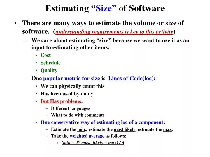
Estimating “Size” of Software • There are many ways to estimate the volume or size of software. (understanding requirements is key to this activity) • We care about estimating “size” because we want to use it as an input to estimating other items: • Cost • Schedule • Quality • One popular metric for size is Lines of Code(loc): • We can physically count this • Has been used by many • But Has problems: • Different languages • What to do with comments • One conservative way of estimating loc of a component: • Estimate the min., estimate the most likely, estimate the max. • Take the weighted average as follows: • (min + 4* most_likely + max) / 6
Cost (Effort)Estimation • In general, effort estimation is based on several parameters and the model ( E= a + b*S**c ): • Personnel • Environment • Quality • Size or Volume of work (e.g. loc) • Process • where S is the Size and a, b, and c are constants estimated with other parameters • a is the base cost needed to perform the project regardless of size • c is the exponent that shows whether the increase of S linearly affects the cost. If c=1 then it is linear. • b is a fixed “marginal” cost per change of S.
Cost/Effort Estimation models • Some popular Effort Estimation methodologies: • Function Point (actually estimates size --- converts to effort) • COCOMO (Constructive Cost Model)
Function Point • Proposed by Albrecht of IBM as an alternative metric to lines of code count for S, size of product. • Based on 5 major areas and a complexity table of (simple, average and complex set of weights: simpleaveragecomplex • input 3 4 6 • output 4 5 7 • inquiry 3 4 6 • master files 7 10 15 • interfaces 5 7 10 • The UnadjustedFunctionPoint (UFP)is : • UFP = w*Inp + w2*Out + w3*Inq + w4*MastF +w5*Intf
Function Point (cont.) • 14 technical complexity factors are included, each “valued” between 0 and 5: • data communications • distributed data • performance criteria • heavy hardware usage • high transaction rates • online data entry • online updating • complex computations • ease of installation • ease of operation • portability • maintainability • end-user efficiency • reusability
Function Point (cont.) • The sum of 14 technical complexity factors can have values of 0 through 70. • The the Total Complexity Factor(TCF) is defined as: • TCF = .65 + (.01 * Sum of 14 technical complexity factors) • Thus TCF may have values of 0.65 through 1.35. • Finally, Function Point (FP) is defined as: FP = UFP * TCF • To convert to effort or cost, one may use “historical” data of productivity and dollars per FP. (need a conversion factor)
Simple Function Point Example • Consider the function that uses ‘Simple” weights from the table : • 2 inputs, 1 output, 0 inquiry, 0 master file, and 2 interfaces • UFP = 3* 2 + 4*1 + 3*0 + 7*0 + 5*2 = 20 • consider the 14 complexity factors : 0-data comm; 0-distrib data; 0-perf criteria; 0-hardware usage; 0-transaction rate; 1-online data entry; 0-end user efficiency; 0-online update; 2-complex computation;0-reusability; 0-ease of install; 0-ease of operation; 0-portability; 1-maintainability: • TCF = .65 + (.01 * 4 ) = .69 • FP = UFP * TCF • FP = 20 * .69 • FP = 13.8
Function Point Example (cont.) • What does 13.8 function points mean in terms of schedule and cost estimates ? • One can receive guidance from IFPUG (International Function Point User Group) to get some of the $/FP or person-days/FP data. • With “old IBM services division” data of 20 function points per person-month to perform “complete” development, 13.8 FP translates to approximately .7 person monthsor (22days * .7 = 15 person days) of work. • Assume $7k/person-month, .7 person months will cost about $5k.
Some Function Points Drawbacks • Requires “trained” people to perform estimates of work volume or product size, especially the 14 technical complexity factors. • While IFPUG may furnish some broader data, Cost and Productivity, figures are still different from organization to organization. • e.g. the IBM data takes into account of corporate “overhead” cost • Some of the 14 Complexity Factors are not that important or complex with today’s tools.
COCOMO Estimating Technique • Developed by Barry Boehm in early 1980’s who had a long history with TRW and government projects (LOC based). Used many projects (~50 some) as the basis. • Later modified into COCOMO II in the mid-1990’s (FP preferred but LOC is still used) • Assumed process activities : • Product Design • Detailed Design • Code and Unit Test • Integration and Test • Utilized by some but most of the software industry people still rely on experience and/or own company proprietary data.
COCOMO I Basic Form for Effort • Effort = A * B * (size ** C) • Effort = person months • A = scaling coefficient • B = coefficient based on 15 parameters • C = a scaling factor for process • Size = delivered source lines of code
COCOMO I Basic form for Time • Time = D * (Effort ** E) • Time = total number of calendar months • D = A constant scaling factor for schedule • E = a coefficient to describe the potential parallelism in managing software development
COCOMO I • Originally based on 56 projects • Reflecting 3 modes of projects • Organic : less complex and flexible process • Semidetached : average project • Embedded : complex, real-time defense projects
3 Modes are Based on 8 Characteristics • A. Team’s understanding of the project objective • B. Team’s experience with similar or related project • C. Project’s needs to conform with established requirements • D. Project’s needs to conform with established interfaces • E. Project developed with “new” operational environments • F. Project’s need for new technology, architecture, etc. • G. Project’s need for schedule integrity • H. Project’s size range
COCOMO I • For the basic forms: • Effort = A * B *(size ** C) • Time = D * (Effort ** E) • Organic : A = 3.2 ; C = 1.05 ; D= 2.5; E = .38 • Semidetached : A = 3.0 ; C= 1.12 ; D= 2.5; E = .35 • Embedded : A = 2.8 ; C = 1.2 ; D= 2.5; E = .32
Coefficient B • Coefficient B is an effort adjustment factor based on 15 parameters which varied from very low, low, nominal, high, very high to extra high • B = Product of (15 parameters) • Product attributes: • Required Software Reliability : .75 ; .88; 1.00; 1.15; 1.40; • Database Size : ; .94; 1.00; 1.08; 1.16; • Product Complexity : .70 ; .85; 1.00; 1.15; 1.30; 1.65 • Computer Attributes • Execution Time Constraints : ; ; 1.00; 1.11; 1.30; 1.66 • Main Storage Constraints : ; ; 1.00; 1.06; 1.21; 1.56 • Virtual Machine Volatility : ; .87; 1.00; 1.15; 1.30; • Computer Turnaround time : ; .87; 1.00; 1.07; 1.15;
Coefficient B (cont.) • Personnel attributes • Analyst Capabilities : 1.46 ; 1.19; 1.00; .86; .71; • Application Experience : 1.29; 1.13; 1.00; .91; .82; • Programmer Capability : 1.42; 1.17; 1.00; .86; .70; • Virtual Machine Experience : 1.21; 1.10; 1.00; .90; ; • Programming lang. Exper. : 1.14; 1.07; 1.00; .95; ; • Project attributes • Use of Modern Practices : 1.24; 1.10; 1.00; .91; .82; • Use of Software Tools : 1.24; 1.10; 1.00; .91; .83; • Required Develop schedule : 1.23; 1.08; 1.00; 1.04; 1.10;
An example • Consider an average project of 10Kloc: • Effort = 3.0 * B * (10** 1.12) = 3 * 1 * 13.2 = 39.6 pm • Where B = 1.0 (all nominal) • Time = 2.5 *( 39.6 **.35) = 2.5 * 3.6 = 9 months • This requires an additional 8% more effort and 36% more schedule time for product plan and requirements: • Effort = 39.6 + (39.6 * .o8) = 39.6 + 3.16 = 42.76 pm • Time = 9 + (9 * .36) = 9 +3.24 = 12.34 months
Some COCOMO I concerns • Is our initial loc estimate accurate enough ? • Are we interpreting each parameter the same way ? • Do we have a consistent way to assess the range of values for each of the 15 parameters ?
COCOMO II • Effort performed at USC with many industrial corporations participating (still guided by Boehm) • Has a database of over 80 some projects • Early estimate, preferred to use Function Point instead of LOC for size; later estimate may use LOC for size. • Coefficient B based on 15 parameters for early estimate is “rolled” up to 7 parameters, and for late estimates use 17 parameters. • Scaling factor for Process has 6 categories ranging in value from .00 to .05, in increments of .01