Download
1 / 22
220 likes | 372 Views
Using Chesapeake Bay Models To Evaluate Dissolved Oxygen Sampling Strategies. Aaron J. Bever, Marjorie A.M. Friedrichs, Carl T. Friedrichs. Outline: Models and data used. Methods of calculating hypoxic volume from 3-dimensional model results

E N D
Using Chesapeake Bay Models To Evaluate Dissolved Oxygen Sampling Strategies Aaron J. Bever, Marjorie A.M. Friedrichs, Carl T. Friedrichs • Outline: • Models and data used. • Methods of calculating hypoxic volume from 3-dimensional model results • How does the number of stations included in the interpolations influence hypoxic volume? • Is improved temporal resolution more important than adding stations? • The models show temporally variable (daily-weekly) DO concentrations and hypoxic volumes. Where do the models recommend the high-frequency data be collected, and how can this high-frequency data help the models? abever@vims.edu 22, February 2011: Chesapeake Bay Program office, Annapolis MD.
Models used: Two 3-D hydrodynamic models with dissolved oxygen • CH3D-ICM: • Complex, multi-component ecosystem model presently used by the CBP. • Extensively calibrate to CBP data. • Model results provided by Ping Wang. • Regional Ocean Modeling System (ROMS) with a one-equation oxygen model: • Constant respiration (no nutrients, primary production, etc.), oxygen saturation at the surface, diffusion of DO, advection of DO with water masses. • No calibration to data. • Model results provided by Malcolm Scully (ODU). • Data used: • Chesapeake Bay Program vertical profiles of DO • Collected bay-wide monthly or bi-monthly • Takes about 7-14 days to sample all stations. • Time-frame of investigation: • Calendar year 2004.
Focusing on hypoxic volume and spatial model estimates of dissolved oxygen. • Hypoxic Volume was calculated from the models in five ways. • Total hypoxic volume from 3D model results. • Hypoxic volume estimated by the model using the observed station locations (snapshot in time). • Hypoxic volume using observed station locations at the exact time each was observed. (directly comparable to the observed hypoxic volume). • Hypoxic volume estimated using all Chesapeake Bay Program stations. • Hypoxic volume estimated using a subset of Chesapeake Bay Program stations and targeted specific locations. • Hypoxic volume was calculated using the Chesapeake Bay Program Visual Basic volume calculator software.
Hypoxic volume calculated from station locations for three of the five methods and the observations. • Absolute Time Match (directly comparable to observations) • Time-snapshot • All Stations
Models suggest estimates of hypoxic volume can be improved through better observing the time-variation in low DO, or DO at strategic locations. • Adding more stations may not improve the estimates of hypoxic volume. • Estimates using all CBP station locations is nearly identical to using the subset actually observed in 2004. • Better resolving the time-variation in low DO will help better estimate hypoxic volume, and better validate/calibrate the models.
Using the model estimates to investigate strategic locations where hypoxia occurs. Fraction of Time Hypoxia Occurred 1-Eq. DO Model ICM Model Chesapeake Bay Program station locations.
Using the model estimates to investigate strategic locations where the variability in DO is high. Standard Deviation of Bottom Oxygen Concentration Choose station locations based on the frequency of hypoxia, variability in DO concentration, and CBP station locations. 1-Eq. DO Model ICM Model Calculate the hypoxic volume based on station subsets to help determine how important different locations are.
Start with a minimum number of stations Selected Station Locations 1-Eq. DO Model
Start with a minimum number of stations Selected Station Locations ICM Model
Include all CBP stations 1-Eq. DO Model Selected Station Locations
Include all CBP stations ICM Model Selected Station Locations
By simply including more stations the hypoxic volume estimated from the stations may have improved, but not as well as hoped. Instead • Strategic placement based on model estimates should help: • Improve the data by using the models to target locations of moderate dissolved oxygen variability near the edge of where hypoxia occurs. • Allows for a more robust estimate of hypoxic volume through time. • Will help examine how the “real” hypoxic volume changes over the 1-2 weeks CBP profiles are being collected. • Helps improve relationships between short-term (daily to weekly) DO forcing factors and the observed DO concentrations. • Improve the models by strategically adding high frequency data to locations where validation is needed. • Near the northern and southern hypoxia extent to determine spatial dimensions through time. • In a known hypoxic region to determine the vertical DO/hypoxia extent through time.
Minimum number of stations: Plus one near the northern hypoxic extent 1-Eq. DO Model ICM Model
Minimum number of stations: Plus one near the south-eastern extent of hypoxia 1-Eq. DO Model ICM Model ICM Model
Improvements in hypoxic volume estimates from adding a station. • Hypoxic volume estimates from the 1-Eq. DO model improved when a single strategic station was added. • Hypoxic Volume estimates from the ICM model were unchanged by adding either of these stations. • Stations on the outer range of hypoxia, and where the variability in DO is high, have the potential to improve estimates of hypoxic volume and significantly contribute to our understanding of the driving forces behind DO concentration within the Chesapeake Bay.
Potential Instrument Locations Based on Model Estimates 1-Eq. model shown; ICM model shows similar results. Northern Bay Middle Bay
Hypoxic volume from the stations and the total estimated hypoxic volume from the 3D fields. 1-Eq. Model
Hypoxic volume from the stations and the total estimated hypoxic volume from the 3D fields. ICM
Spatial model estimated bottom DO concentration (mg/L). 1-Eq. Model 2 mg/L is contoured in black.
Spatial model estimated bottom DO concentration (mg/L). ICM model: Much more calibrated to observed profiles, much less variable than 1-Eq. 2 mg/L is contoured in black. X and Y axis are in UTM, per ICM output.