Download
1 / 29
290 likes | 308 Views
This study examines the kinetic structure of the reconnection layer and slow mode shocks in the context of collisionless reconnection in thin current sheets. The analysis includes simulations, equilibrium setup, development of the reconnection line and channels, and investigation of slow mode shocks.

E N D
Kinetic Structure of the Reconnection Layer and of Slow Mode Shocks Manfred Scholer Centre for Interdisciplinary Plasma Science Max-Planck-Institut für extraterrestrische Physik, Garching, Germany Kaspar Arzner Michael Cremer Irina Sidorenko Isaac Newton Institute, August 2004
First a few vgiewgraphs about Onset of collisionless reconnection in thin current sheets: Anti-parallel and sheared magnetic fields (3-D PIC simulations) Scholer, Sidorenko, Jaroschek, Treumann, 2003
Initial Equilibrium and Numerical Set-up Double Harris-sheet Current sheet width = 1 ion inertial length Periodicity in all three directions particles of each species (note the coordinate system: z is the current direction)
I. Thin Current Sheet with Antiparallel Magnetic Field Right: Reconnected flux versus time. The whole flux between the two current sheets is reconnected when Left: Magnetic field pattern at four different times (Isointensity contours of )
Lower Hybrid Drift Instability at the Current Sheet Edge Color coded electron density (left) and electric field (right) in the current directionin the plane perpendicular to the magnetic field.
Cuts of various parameters before reconnection starts t=0 t=4 Cuts of electron contribution to current density (top) and electron density across the current sheet. Profiles at t=0 are shown dashed for reference. Reduced electron distribution function f(v_z) versus v_z in the current sheet gradient region (top) and in the center (bottom) of the current sheet exhibiting electron acceleration in the electric field of the LHD waves.
Developmentof the Reconnection Line Reconnecrtion channel Shown is the normal magnetic field component in the center of the current sheet (blue: negative field, red: positive field). Transitions from red to blue indicate positions of a neutral line. Initially, several single neutral lines emerge. Eventually one single reconnection channel results. Two reconnection channels
Development of Neutral Line (Guide Field Case Bz=1) With a sufficiently strong guide field reconnection is two-dimensional, i.e., a single X line develops and extends through the whole system Time for electrons to move across the system smaller than growth time of instability
Guide Field = 20% of Main Field Deviation of main field above (right) and below (left) current sheet at wo different times LH waves propagate perpendicular to the Magnetic field In this guide field case the LHDI develops as well. After reconnection onset the reconnection rate is about the same as in the exactly antiparallel case.
Developmentof the Reconnection Channels Guide field = 0.2 of main field
‘Antiparallel reconnection‘ ‘Component reconnection‘
Reconnection Layer Collisionless MHD Petschek, 1964 2 switch-off shocks bound the reconnection layer Hill, 1975 Current sheet where particles Perform Speiser-type orbits
Investigation of the reconnection layer by large-scale hybrid • simulations • Analysis of slow mode shocks by solving an equivalent Riemann • problem (decay of a current sheet)
2-D hybrid simulation of tail reconnection Hybrid code with massless electrons Initial equilibrium is Birn et al. (1975) equilibrium with flaring tail (but can also be a Harris sheet) Simulation box of 500 x 126 ion inertial lengths (lO=c/wpi , where plasma frequency refers to current sheet center density) (corresponds to about 100 x 25 RE) Lobe density to center density at x=0 is 0.4 Temperature is chosen such that overall prssure balance is maintained (bi=be=0.05 in the lobe) Reconnection is initialized by localized resistivity at 100 lO Computed up to 500 Wci-1 We are back to the magnetospheric coordinare system
By – field (out-of-plane) y-component of ion vorticity is frozen into ion fluid u. In the inflow lobe region both terms are zero. Occurrence of vorticity has to be cancelled by By
1.Near diffusion region: interpenetrating cold beams 2.Center of current sheet: Partial ring distribution due to Speiser-type orbitsin CS with thickness larger than ion gyroradius 3.Boundary layer: Speiser accelerated ions ejected onto reconnected field lines 4.Post-plasmoid plasma sheet: Hot thermalized distribution 1.,2.,3. closely resembles Hill (1975) scenario
Instability and breakup of current sheet Waves are standing in the outflow frame
Instability and breakup of the current sheet Bulk velocity shear insufficient to drive KH instability. Beams in the BL provide additional energy to drive instabiliy. Due to sharp gradients in BL a homogeneous scenario does not apply. 3-layer anisotropic MHD model. Free energy mainly produced by velocity anisotropy; bulk velocity shear plays auxiliary role
Comparison of solution of dispersion relation with simulation Arzner and Scholer, 2001 Simulation: Dominant wavelength l = 20 lO, corresponding to k = 0.3; wavelength increases with x. Phase velocity and group velocity about equal to outflow velocity. 3-layer model (red) compares favorably with simulation.
Development of the instability with distance higher harmonics cascading to lower wavelengths monochromatic
Simulated power spectra of B time series averaged over the turbulent range in the post plasmoid plasma sheet. Agrees with observed temporal power spectra in the tail (AMPTE: Bauer et al., 1995; GEOTAIL: Hoshino et al., 1994).
Hot thermalized post-plasmoid plasma sheet Boundary layer Lobe distribution
Dissipation Mechanism in Slow Mode Shocks Bounding the Reconnection Layer Cremer and Scholer, 2000
Solution of an Equivalent Riemann Problem (Decay of a 1D current sheet wit normal magnetic field)
Perpendicular Heating of Lobe by the EMIIC Instability Ion distribution function In the LOBE! Temperature in lobe vs time
Nonresonant and right-hand resonant ion-ion beam instabilities are stable. Oblique propagating AIC waves are excited by the EMIIC instability. They heat lobe and beam ions perpendicular to the magnetic field. Large perpendicular to parallel temperature anisotropy excites parallel propagating AIC waves. These AIC waves lead downstream to ion phase-mixing and thermalization.
Excitation of parallel propagating AIC waves by the perp to parallel temperature anisotropy W-kxpower spectrum and result from linear theory; hodogram of kx=1 mode 2D Fourier analysis in the kx-kzplane
Suggested cycle of processes leading to slow mode shocks bounding the reconnection layer