Download
1 / 32
320 likes | 334 Views
A hybrid quantization scheme for image compression. Source : Image and Vision Computing, Vol: 22, Issue: 3, pp. 203-213, March 1, 2004 Author : Paul Shelley, Xiaobo Li, Bin Han Speaker : Chang-Chu Chen Date : 6/1/2004. Outline. Image compression based on Wavelet

E N D
A hybrid quantization scheme for image compression Source : Image and Vision Computing, Vol: 22, Issue: 3, pp. 203-213, March 1, 2004 Author : Paul Shelley, Xiaobo Li, Bin Han Speaker : Chang-Chu Chen Date : 6/1/2004
Outline • Image compression based on Wavelet • SPIHT and ModLVQ • Proposed scheme • Results • Conclusions
Image compression based on Wavelet Original image Wavelet coefficients Quantization Coding 10 11 0 0 1 10 0 0 0 1 0 0 0 0 0 0 1 0 1 0 10 0 0 0 0 1010 EZW, SPIHT, ModLVQ…
Subband LL3 HL3 LL3 HL3 HL2 HL2 LH3 HH3 LH3 HH3 LL1 HL1 HL1 LL1 LH2 HH2 LH2 HH2 LH1 HH1 LH1 HH1
Quadtree LL2 X X LL2 HL2 X HL1 LH2 HH2 LH2 Y Y Y LH1 HH1 LH1
Zerotree Tk : kth threshold DWT coefficients
SPIHT and ModLVQ • Set Partitioning in Hierarchical Trees • Modified lattice vector quantization 2x2 blocks 4x4 blocks Zerotree Threshold Tk+1 = 0.5 * Tk Zerotree Threshold Tk+1 = 0.65 * Tk
SPIHT and ModLVQ(cont.) Smooth image Detailed image
SPIHT and ModLVQ(cont.) Smooth image Detailed image
Proposed Scheme • Hy-Q (Hybrid Quantization) Smooth subimage SPIHT divide image to subimages ModLVQ Detailed subimage
Proposed Scheme (cont.) Threshold 0.94
Results (cont.) • For uniformly smooth or uniformly detailed images, Hy-Q provides over 85% of the time. • For some feature quadrants are mostly smooth and the others are mostly detailed, Hy-Q provides over 77% of the time.
Conclusions • Proposed a new algorithm Hy-Q for the quantization step of wavelet image compression. • Proposed scheme mixes two quantization strategies : • SPIHT is used for quantize the smooth regions. • ModLVQ is used for quantize the detailed regions.
Discrete Wavelet Transform -Haar Phase 1) Horizontal: Phase 2) Vertical:
Discrete Wavelet Transform -Haar(cont.) Example Phase 1) Horizontal: Level one Phase 2) Vertical: (Level one is done) Phase 1) Horizontal: Level two Phase 2) Vertical: (Level two is done)
LL2 HL2 LL1 HL1 LH2 HH2 LH1 HH1 Discrete Wavelet Transform -Haar(cont.) Example 1” Wavelet 2” Wavelet
SPIHT • Notationsn :H : Set of coordinates of all spatial orientation tree rootsLSP : List of significant pixelsLIP : List of insignificant pixelsLIS : List of insignificant Sets type A : Set of coordinates of all descendants of a node type B : Set of coordinates of all descendants of a node, but not include this node
SPIHT algorithm Output: n= 5 // 25=32 (threshold T0 ) H=(0,0), (1,0), (0,1), (1,1) // head (roots of trees) LIP: (0,0)→(0,1)→(1,0)→(1,1) LIS: LSP:
SPIHT algorithm (cont.) Output: 63 –34 –31 23 10(+) 11(-) 0 0 n= 5 // 25=32 (threshold T0 ) H=(0,0), (1,0), (0,1), (1,1) // head (roots of trees) LIP: (0,0)→(0,1)→(1,0)→(1,1) X X R R LIS: A(0,1)→A(1,0)→A(1,1) LSP: (0,0) (0,1)
SPIHT algorithm (cont.) Output: 63 –34 –31 23 A(0,1) 49 10 14 –13 10(+) 11(-) 0 0 1 10 0 0 0 n= 5 // 25=32 (threshold T0 ) H=(0,0), (1,0), (0,1), (1,1) // head (roots of trees) LIP: (0,0)→(0,1)→(1,0)→(1,1) →(0,2) →(0,3) →(1,2) →(1,3) X X R R X R R R LIS: A(0,1)→A(1,0)→A(1,1) →B(0,1) X LSP: (0,0) (0,1) (0,2)
SPIHT algorithm (cont.) Output: 63 –34 –31 23 A(0,1) 49 10 14 –13 A(1,0) 15 14 –9 -7 10(+) 11(-) 0 0 1 10 0 0 0 1 0 0 0 0 n= 5 // 25=32 (threshold T0 ) H=(0,0), (1,0), (0,1), (1,1) // head (roots of trees) LIP: (0,0)→(0,1)→(1,0)→(1,1) →(0,2) →(0,3) →(1,2) →(1,3) →(2,0) →(2,1) →(3,0) →(3,1) X X R R X R R R R R R R LIS: A(0,1)→A(1,0)→A(1,1) →B(0,1) →B(1,0) X X LSP: (0,0) (0,1) (0,2)
SPIHT algorithm (cont.) Output: 63 –34 –31 23 A(0,1) 49 10 14 –13 A(1,0) 15 14 –9 -7 A(1,1) 10(+) 11(-) 0 0 1 10 0 0 0 1 0 0 0 0 0 n= 5 // 25=32 (threshold T0 ) H=(0,0), (1,0), (0,1), (1,1) // head (roots of trees) LIP: (0,0)→(0,1)→(1,0)→(1,1) →(0,2) →(0,3) →(1,2) →(1,3) →(2,0) →(2,1) →(3,0) →(3,1) X X R R X R R R R R R R LIS: A(0,1)→A(1,0)→A(1,1) →B(0,1) →B(1,0) X X R LSP: (0,0) (0,1) (0,2)
SPIHT algorithm (cont.) Output: 63 –34 –31 23 A(0,1) 49 10 14 –13 A(1,0) 15 14 –9 -7 A(1,1) 10(+) 11(-) 0 0 1 10 0 0 0 1 0 0 0 0 0 B(0,1) 0 n= 5 // 25=32 (threshold T0 ) H=(0,0), (1,0), (0,1), (1,1) // head (roots of trees) LIP: (0,0)→(0,1)→(1,0)→(1,1)→(0,2)→(0,3)→(1,2)→(1,3)→(2,0)→(2,1)→(3,0)→(3,1) X X R R X R R R R R R R LIS: A(0,1)→A(1,0)→A(1,1)→B(0,1) X X R R LSP: (0,0) (0,1) (0,2)
SPIHT algorithm (cont.) Output: 63 –34 –31 23 A(0,1) 49 10 14 –13 A(1,0) 15 14 –9 -7 A(1,1) 10(+) 11(-) 0 0 1 10 0 0 0 1 0 0 0 0 0 B(0,1) B(1,0) 0 1 n= 5 // 25=32 (threshold T0 ) H=(0,0), (1,0), (0,1), (1,1) // head (roots of trees) LIP: (0,0)→(0,1)→(1,0)→(1,1)→(0,2)→(0,3)→(1,2)→(1,3)→(2,0)→(2,1)→(3,0)→(3,1) X X R R X R R R R R R R LIS: A(0,1)→A(1,0)→A(1,1)→B(0,1)→B(1,0)→A(2,0)→A(2,1)→A(3,0)→A(3,1) X X R R R LSP: (0,0) (0,1) (0,2)
SPIHT algorithm (cont.) Output: 63 –34 –31 23 A(0,1) 49 10 14 –13 A(1,0) 15 14 –9 -7 A(1,1) 10(+) 11(-) 0 0 1 10 0 0 0 1 0 0 0 0 0 B(0,1) B(1,0) A(2,0) 0 1 0 n= 5 // 25=32 (threshold T0 ) H=(0,0), (1,0), (0,1), (1,1) // head (roots of trees) LIP: (0,0)→(0,1)→(1,0)→(1,1)→(0,2)→(0,3)→(1,2)→(1,3)→(2,0)→(2,1)→(3,0)→(3,1) X X R R X R R R R R R R LIS: A(0,1)→A(1,0)→A(1,1)→B(0,1)→B(1,0)→A(2,0)→A(2,1)→A(3,0)→A(3,1) X X R R R R LSP: (0,0) (0,1) (0,2)
SPIHT algorithm (cont.) Output: 63 –34 –31 23 A(0,1) 49 10 14 –13 A(1,0) 15 14 –9 -7 A(1,1) 10(+) 11(-) 0 0 1 10 0 0 0 1 0 0 0 0 0 B(0,1) B(1,0) A(2,0) A(2,1) –1 47 –3 –2 0 1 0 1 0 10 0 0 n= 5 // 25=32 (threshold T0 ) H=(0,0), (1,0), (0,1), (1,1) // head (roots of trees) LIP: (0,0)→(0,1)→(1,0)→(1,1)→(0,2)→(0,3)→(1,2)→(1,3)→(2,0)→(2,1)→(3,0)→(3,1)→ X X R R X R R R R R R R (4,2)→(4,3)→(5,2)→(5,3) R X R R LIS: A(0,1)→A(1,0)→A(1,1)→B(0,1)→B(1,0)→A(2,0)→A(2,1)→A(3,0)→A(3,1) X X R R R R X LSP: (0,0) (0,1) (0,2) (4,3)
SPIHT algorithm (cont.) Output: 63 –34 –31 23 A(0,1) 49 10 14 –13 A(1,0) 15 14 –9 -7 A(1,1) 10(+) 11(-) 0 0 1 10 0 0 0 1 0 0 0 0 0 B(0,1) B(1,0) A(2,0) A(2,1) –1 47 –3 –2 A(3,0) 0 1 0 1 0 10 0 0 0 n= 5 // 25=32 (threshold T0 ) H=(0,0), (1,0), (0,1), (1,1) // head (roots of trees) LIP: (0,0)→(0,1)→(1,0)→(1,1)→(0,2)→(0,3)→(1,2)→(1,3)→(2,0)→(2,1)→(3,0)→(3,1)→ X X R R X R R R R R R R (4,2)→(4,3)→(5,2)→(5,3) R X R R LIS: A(0,1)→A(1,0)→A(1,1)→B(0,1)→B(1,0)→A(2,0)→A(2,1)→A(3,0)→A(3,1) X X R R R R X R LSP: (0,0) (0,1) (0,2) (4,3)
SPIHT algorithm (cont.) Output: 63 –34 –31 23 A(0,1) 49 10 14 –13 A(1,0) 15 14 –9 -7 A(1,1) 10(+) 11(-) 0 0 1 10 0 0 0 1 0 0 0 0 0 B(0,1) B(1,0) A(2,0) A(2,1) –1 47 –3 –2 A(3,0) A(3,1) 0 1 0 1 0 10 0 0 0 0 n= 5 // 25=32 (threshold T0 ) H=(0,0), (1,0), (0,1), (1,1) // head (roots of trees) LIP: (0,0)→(0,1)→(1,0)→(1,1)→(0,2)→(0,3)→(1,2)→(1,3)→(2,0)→(2,1)→(3,0)→(3,1)→ X X R R X R R R R R R R (4,2)→(4,3)→(5,2)→(5,3) R X R R LIS: A(0,1)→A(1,0)→A(1,1)→B(0,1)→B(1,0)→A(2,0)→A(2,1)→A(3,0)→A(3,1) X X R R R R X R R LSP: (0,0) (0,1) (0,2) (4,3)
SPIHT algorithm (cont.) Refine the set LSP (0,0) (0,1) (0,2) (4,3) according to the refinement of EZW and generate 1010 Output: 10 11 0 0 1 10 0 0 0 1 0 0 0 0 0 0 1 0 1 0 10 0 0 0 0 1010