Download
1 / 28

E N D
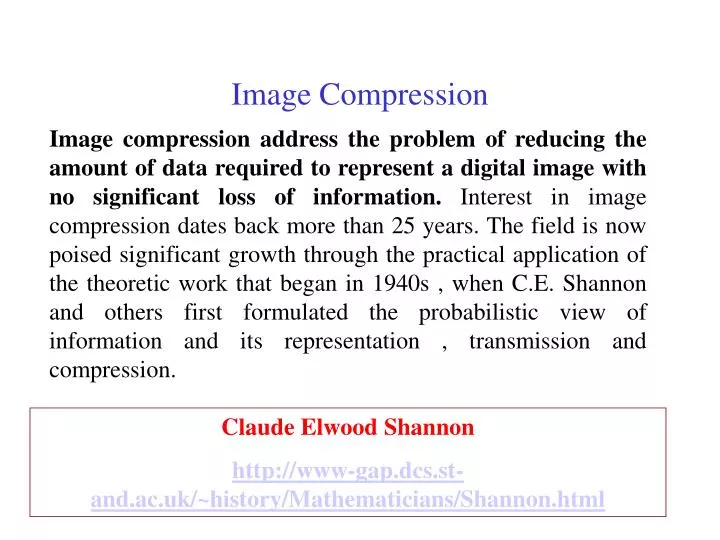
Image Compression Image compression address the problem of reducing the amount of data required to represent a digital image with no significant loss of information. Interest in image compression dates back more than 25 years. The field is now poised significant growth through the practical application of the theoretic work that began in 1940s , when C.E. Shannon and others first formulated the probabilistic view of information and its representation , transmission and compression. Claude Elwood Shannon http://www-gap.dcs.st-and.ac.uk/~history/Mathematicians/Shannon.html
Image Compression Images take a lot of storage space: - - 1024 x 1024 x 32 x bits images requires 4 MB - - suppose you have some video that is 640 x 480 x 24 bits x 30 frames per second , 1 minute of video would require 1.54 GB Many bytes take a long time to transfer slow connections – suppose we have 56,000 bps - - 4MB will take almost 10 minutes - - 1.54 GB will take almost 66 hours Storage problems, plus the desire to exchange images over the Internet, have lead to a large interest in image compression algorithms.
The same information can be represented many ways. Data are the means by which information is conveyed. Various amounts of data can be used to convey the same amount of information. Example: Four different representation of the same information ( number five) 1) a picture ( 1001,632 bits ); 2) a word “five” spelled in English using the ASCII character set ( 32 bits); 3) a single ASCII digit ( 8bits); 4) binary integer ( 3bits)
Compression algorithms remove redundancy If more data are used than is strictly necessary, then we say that there is redundancy in the dataset. Data redundancy is not abstract concept but a mathematically quantifiable entity . If n1 and nc denote the number of information carrying units in two data sets that represent the same information, the relative data redundancyRD of the first data set ( n1 ) can be defined as RD= 1 – 1/CR (1) Where CRis compression ration, defined as CR = n1/nc (2) Where n1 is the number of information carrying units used in the uncompressed dataset and nc is the number of units in the compressed dataset. The same units should be used for n1 and nc; bits or bytes are typically used. When nc<<n1 , CR large value and RD 1. Larger values of C indicate better compression
A general algorithm for data compression and image reconstruction Input image ( f(x,y) Reconstructed image f’(x,y) Source decoder Reconstruction Source encoder Data redundancy reduction Channel Channel encoder Channel decoder An input image is fed into the encoder which creates a set of symbols from the input data. After transmission over the channel, the encoded representation is fed to the decoder, where a reconstructed output image f’(x,y) is generated . In general , f’(x,y) may or may not an exact replica of f(x,y). If it is , the system is error free or information preserving, if not, some level of distortion is present in the reconstructed image .
Data compression algorithms can be divided into two groups : 1 Lossless algorithms remove only redundancy present in the data . The reconstructed image is identical to the original , i.e., all af the information present in the input image has been preserved by compression . 2. Higher compression is possible using lossy algorithms which create redundancy (by discarding some information ) and then remove it .
Fidelity criteria When lossy compression techniques are employed, the decompressed image will not be identical to the original image. In such cases , we can define fidelity criteria that measure the difference between this two images. Two general classes of criteria are used : (1) objective fidelity criteria and (2) subjective fidelity criteria A good example for (1) objective fidelity criteria is root-mean square ( RMS ) error between on input and output image For any value of x,and y , the error e(x,y) can be defined as : e(x,y) = f’(x,y) – f(x,y) The total error between two images is: The root –mean square error , erms is :
Types of redundancy • Three basic types of redundancy can be identified in a single image: • Coding redundancy • Interpixel redundancy • Psychovisual redundancy
Coding redundancy • our quantized data is represented using codewords • The codewords are ordered in the same way as the intensities that they represent; thus the bit pattern 00000000, corresponding to the value 0, represents the darkest points in an image and the bit pattern 11111111, corresponding to the value 255, represents the brightest points. • if the size of the codeword is larger than is necessary to represent all quantization levels, then we have coding redundancy • An 8-bit coding scheme has the capacity to represent 256 distinct levels of intensity in an image . But if there are only 16 different grey levels in a image , the image exhibits coding redundancy because it could be represented using a 4-bit coding scheme. Coding redundancy can also arise due to the use of fixed-length codewords.
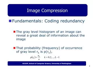
Grey level histogram of an image also can provide a great deal of insight into the construction of codes to reduce the amount of data used to represent it . Let us assume, that a discrete random variable rk in the interval (0,1) represents the grey levels of an image and that each rk occurs with probability Pr(rk). Probability can be estimated from the histogram of an image using Coding redundancy Pr(rk) = hk/n for k = 0,1……L-1 (3) Where L is the number of grey levels and hk is the frequency of occurrence of grey level k (the number of times that the kth grey level appears in the image) and n is the total number of the pixels in the image. If the number of the bits used to represent each value of rk is l(rk), the average number of bits required to represent each pixel is : (4)
Rk Pr(rk) Code 1 l1(rk) Code 2 l2(rk) r0 = 0 0.19 000 3 11 2 r1 = 1/7 0.25 001 3 01 2 r2 = 2/7 021 010 3 10 2 r3 = 3/7 0.16 011 3 001 3 r4 = 4/7 0.08 100 3 0001 4 r5 = 5/7 0.06 101 3 00001 5 r6 = 6/7 0.03 110 3 000001 6 r7=1 0.02 111 3 000000 6 Coding redundancy - Example Using eq. (2) the resulting compression ratio Cn is 3/2.7 or 1.11 Thus approximately 10 percent of the data resulting from the use of code 1 is redundant. The exact level of redundancy is RD = 1 – 1/1.11 =0.099
Interpixel redundancy The intensity at a pixel may correlate strongly with the intensity value of its neighbors. Because the value of any given pixel can be reasonably predicted from the value of its neighbors Much of the visual contribution of a single pixel to an image is redundant; it could have been guessed on the bases of its neighbors values. We can remove redundancy by representing changes in intensity rather than absolute intensity values .For example , the differences between adjacent pixels can be used to represent an image . Transformation of this type are referred to as mappings. They are called reversible if the original image elements can be reconstructed from the transformed data set. For example the sequence (50,50, ..50) becomes (50, 4).
Psychovisual redundancy Example First we have a image with 256 possible gray levels . We can apply uniform quantization to four bits or 16 possible levels The resulting compression ratio is 2:1. Note , that false contouring is present in the previously smooth regions of the original image. The significant improvements possible with quantization that takes advantage of the peculiarities of the human visual system . The method used to produce this result is known as improved gray-scale ( IGS) quantization. It recognizes the eye’s inherent sensitivity to edges and breaks them up by adding to each pixel a pseudo-random number, which is generated from the order bits of neighboring pixels, before quantizing the result.
Error free compression Delta compression ( differential coding ) is a very simple, lossless techniques in which we recode an image in terms of the difference in gray level between each pixel and the previous pixel in the row. The first pixel must be represented as an absolute value, but subsequent values can be represented as differences , or ‘deltas”. For example: FIGURE :Example of delta encoding. The first value in the encoded file is the same as the first value in the original file. Thereafter, each sample in the encoded file is the difference between the current and last sample in the original file.
Delta compression FIGURE:Example of delta encoding. Figure (a) is an audio signal digitized to 8 bits. Figure (b) shows the delta encoded version of this signal. Delta encoding is useful for data compression if the signal being encoded varies slowly from sample-to-sample. Takes advantage of interpixel redundancy in a scan line
CTRL COUNT CHAR Also take advantage of interpixel redundancy . Run length encoding A “run: of consecutive pixels whose gray levels are identical is replaced with two values: the length of the run and the gray level of all pixels in the run. Exampe ( 50, 50,50,50) becomes (4,50) Especially suited for synthetic images containing large homogeneous regions . The encoding process is effective only if there are sequences of 4 or more repeating characters Applications – compression of binary images to be faxed. CTRL - control character which is used to indicate compressionCOUNT- number of counted characters in stream of the same charactersCHAR - repeating characters FIGURE:. Format of three byte code word
Examples of RLE implementations RLE algorithms are parts of various image compression techniques like BMP, PCX, TIFF, and is also used in PDF file format, but RLE also exists as separate compression technique and file format. MS Windows standard for RLE have the same file format as well-known BMP file format, but it's RLE format is defined only for 4-bit and 8-bit color images.Two types of RLE compression is used 4bit RLE and 8bit RLE as expected the first type is used for 4-bit images, second for 8-bit images.
Second byte Definition 0 End-of-line 1 End-of-Rle(Bitmap) 2 Following two bytes defines offset in x and y direction (x is right,y is up). The skipped pixels get color zero. >=3 when expanding following >=3 nibbles (4bits) are just copied from compressed file, file/memory pointer must be on 16bit boundary so adequate number of zeros follows 4bit RLE Compression sequence consists of two bytes, first byte (if not zero) determines number of pixels which will be drawn. The second byte specifies two colors, high-order 4 bits (upper 4 bits) specifies the first color, low-order 4bits specifies the second color this means that after expansion 1st, 3rd and other odd pixels will be in color specified by high-order bits, while even 2nd, 4th and other even pixels will be in color specified by low-order bits. If first byte is zero then the second byte specifies escape code. (See table below)
Compressed data Expanded data 06 52 5 2 5 2 5 2 08 1B 1 B 1 B 1 B 1 B 00 06 83 14 34 8 3 1 4 3 4 00 02 09 06 Move 9 positions right and 6 up 00 00 End-of –line 04 22 2 2 2 2 00 01 End-of-RLE(Bitmap) Examples for 4bit RLE:
8bit RLE Sequence when compressing is also formed from 2 bytes, the first byte (if not zero) is a number of consecutive pixels which are in color specified by the second byte.Same as 4bit RLE if the first byte is zero the second byte defines escape code, escape codes 0, 1, 2, have same meaning as described in Table 1. while if escape code is >=3 then when expanding the following >=3 bytes will be just copied from the compressed file, if escape code is 3 or other greater odd number then zero follows to ensure 16bit boundary.
Compressed data Expanded data 06 52 52 52 52 52 52 52 08 1B 1B 1B 1B 1B 1B 1B 1B 1B 00 03 83 14 34 83 14 34 00 02 09 06 Move 9 positions right and 6 up 00 00 End-of -line 04 2A 2A 2A 2A 2A 00 01 End-of-RLE(Bitmap) Examples for 8bit RLE
Statistical coding Statistical coding techniques remove the coding redundancy in an image. Information theory tells us that the amount of information conveyed by a codeword relates to its probability of occurrence. Codeword that occur rarely convey more information that codeword that occur frequently in the data. A random event i that occurs with probability P(i) is said to contain I(i) = -logP(i) units of information ( self information ) If P(i) = 1 ( that is, the event always occurs) I(i) = 0 and no information is attributed to it . Let us assume that information source generates a random sequence of symbols ( grey level). The probability of occurrence for a grey level i is P(i) . If we have 2b-1 gray level ( symbols ) the average self-information obtained from i outputs is called entropy.
Entropy in information theory is the measure of the information content of a message. Entropy gives a average bits per pixel required to encode an image. Probabilities are computed by normalizing the histogram of the image – P(i)=hi/n Where hi is the frequency of occurrence of grey level i and n is the total number of pixels in the image. If bis the smallest number of bits needed to generate a number of quatisation levels observed in an image, then the information redundancy of that image is defined as R =b-H The compression ratio is Cmax= b/H
Statistical coding • After computing the histogram and normalizing the task is to construct a set of codewords to represent each pixel value . These codewords must have the following properties: • Different codewords must have different lengths ( number of bits0 • Codewords that occurs infrequently ( low probability ) should use more bits. Codewords that occur frequently ( high probability ) should use fewer bits. • It must not be possible to mistake a particular sequence of concatenated codewords for any other sequence. • The average bit length of codewords is where l(i) is the length of the codeword used to represent the grey level i. From Shannon first coding theorem the upper limit for Lavg is b and the lower limit for Lavg is the entropy.
Huffman coding • Ranking pixel values in decreasing order of their probability • Pair the two values with the lowest probabilities, labeling one of them with 0 and other with 1. • Link two symbols with lowest probabilities . • Go to step 2 until you generate a single symbol which probability is 1. • Trace the coding tree from a root. http://www.compressconsult.com/huffman/ http://www.cs.duke.edu/csed/poop/huff/info/
Dictionary –based coding The methods of the first group try to find if the character sequence currently being compressed has already occurred earlier in the input data and then, instead of repeating it, output only a pointer to the earlier occurrence. http://www.rasip.fer.hr/research/compress/algorithms/fund/lz/lz77.html)
Dictionary –based coding The algorithms of the second group create a dictionary of the phrases that occur in the input data. When they encounter a phrase already present in the dictionary, they just output the index number of the phrase in the dictionary. This is explained in the diagram below: