Download
1 / 74
860 likes | 950 Views
Model Parameterization and Validation. Prof. Cesar de Prada Dpt. Systems Engineering and Automatic Control University of Valladolid prada@autom.uva.es. Outline. Introduction Parameterization / Calibration Sensitivities Identifiability Dynamic optimization Model validation.

E N D
Model Parameterization and Validation Prof. Cesar de Prada Dpt. Systems Engineering and Automatic Control University of Valladolid prada@autom.uva.es
Outline • Introduction • Parameterization / Calibration • Sensitivities • Identifiability • Dynamic optimization • Model validation Cesar de Prada ISA-UVA
Modelling Methodology Process knowledge There are specific methods and tools to facilitate the implementation of these steps Aims, Model kind Hypothesis Model formulation Parameter estimation Model Evaluation time Explotation Cesar de Prada ISA-UVA
Simulation Tools Hypothesis Range of validity Knowledge Model aims, required precision,… Modelling Coding Simulation language Formulation for a specific calculation Parameterization Experimentation All stages must be validated Is it adequately solved? Validation/ Experimentation Cesar de Prada ISA-UVA
Modelling • Two steps: • Model structure building • Estimating the value of the model parameters Generally, a choice among different possible model structures must be made, in agreement with the selected hypothesis At the validation stage, several test can be proposed to select the best option Cesar de Prada ISA-UVA
Parameterization Some model parameters can be obtained from bibliography, documentation, etc. but there are always other ones that must be estimated from experimental data. Cesar de Prada ISA-UVA
Example: Chemical reactor A TT AB Reactor Coolant AT Product Cesar de Prada ISA-UVA
Parameterization (calibration) A TT u Reactor Coolant AT t Product y y u pa Model pb Given a set of inputs, the model response depends on the value of the parameters p p Cesar de Prada ISA-UVA
Parameterization (calibration) If N measurements yp(t) of the process output have been collected, it is possible to define the error function: u y(p) yp(t) y u Model y(u,p,t) p t Other formulations can be made also for J Cesar de Prada ISA-UVA
Parameterization (calibration) v yp u Process e(t) Optimization Model y(p) p J normally is a non-linear function of the parameters p, and the problem must be solved numerically using DO methods. Cesar de Prada ISA-UVA
Dynamic model parameterization Dynamic optimization with constraints problem, DO Besides the explicit model parameters, unknown initial states , disturbances or non measured inputs can also be included in the parameter estimation problem. Cesar de Prada ISA-UVA
Parameterization Process Generally, there are several measured process outputs: y Attention should be paid to avoid mixing variables with different units and orders of magnitude. Normalization is required. Weights reflect relative importance Cesar de Prada ISA-UVA
Other possible cost functions Norm 1 All errors are equally weighted Norm Minimizes the largest error Weighted LS Errors are weighted inversely to the noise present in the data Cesar de Prada ISA-UVA
Data reconciliation • Data reconciliation intends to: • Estimate the values of all variables and model parameters coherent with a process model and as close as possible to the measurements • Detect and correct inconsistencies in the measurements Cesar de Prada ISA-UVA
Robust estimators Fair function Welsch Cesar de Prada ISA-UVA
Robust estimators c > b +2a Hampel’s Redescending estimator R a, b, c tuning parameters Smoothing functions Cesar de Prada ISA-UVA
Which parameters should be estimated? It may happen that the model response to a given set of inputs for two values p1 and p2 of a certain parameter does not change in a significant way. A parameter should be included in the optimization only if the model output presents a sensible sensitivity to changes in the parameter. u y p1 p2 Cesar de Prada ISA-UVA
Output sensitivitiesCost function sensitivity Sensitivity of cost function J with respect to parameter j in a given experiment. Summarize the effect of the parameter change over the whole experiment. Sensitivity of the model output i with respect to parameter j in a given experiment. Notice that it is a time function. Cesar de Prada ISA-UVA
Output sensitivities It is difficult to compare output sensitivities due to the different units in which they are expressed. It is better to use relative sensitivities The norm of column j of the output sensitivity matrix provides a measure of the importance of parameter pj in the value of the model outputs. Cesar de Prada ISA-UVA
Computing output sensitivities They can be obtained using finite differences approximation or integrating the extended system. One option is to use model simulations with small perturbations on each parameter involved The value of the sensitivities obtained depends on the point p considered and the experiment that was performed as u(t) is involved in the simulations. Cesar de Prada ISA-UVA
Extended system sensitivities Integrating this equation, besides the ones of the model, it is possible to obtain the time evolution of the sensitivities x/p and, hence, the output sensitivities. IDAS Cesar de Prada ISA-UVA
Example: Heated tank Ti T temperature m tank mass h liquid level V voltage q Inflow F Outflow a valve opening H entalphy ce specific heat A tank cross section • density R resistence Te external temperature Ti inflow temperature q Te m V R T h F a Hypothesis: T lumped temperature constant density ce constant specific heat Cesar de Prada ISA-UVA
Ti q Te m V R T h F a Dynamic model State space non-linear model CV: T temperature MV: V voltage h level a valve opening Disturbances: q Inflow, Ti Input temperature States: h , T Other variables: F outflow Cesar de Prada ISA-UVA
Sensitivities h T A Uamb R k Cesar de Prada ISA-UVA
Identifiability We say a model is identifiable if it is possible to obtain the value of its parameters provided that sufficient number of process measurements is available. In practice, identifiability means that a certain model output corresponds to a certain value of the parameter set. But it may happens that the same effect on the output can be attained either modifying one parameter or another. In this case, there is a certain co-linearity in that parameter set which makes very difficult the identification. Identifiability is a structural property of the model, but the identification of particular parameter can depend also on the experimental data. Cesar de Prada ISA-UVA
Identifiability examples In a chemical reactor, without temperature measurements, parameters k and E, cannot be estimated independently In the model, it is possible to identify the ratio F/V, but not F and V independently. With steady state data, V cannot be identified. In the Monod model, using data limited to small values of s, only the ratio m/K can be identified. With data containing only large values of s, only m can be identified well. s Cesar de Prada ISA-UVA
Identifiability With the output sensitivity matrix, it is possible to see if a certain degree of co-linearity exists, by inspecting range of its sub-blocks (by rows). sij sik t Co-linearity makes parameter identification more difficult Cesar de Prada ISA-UVA
Re-parameterization Sometimes it is only possible to identify certain parameter combinations, or new variables can be defined in the model to obtain a model structure easier to identify. If either of these alternatives has been implemented, it is necessary to remember that: • Statistical characteristics of new variables are different to the ones of the data set. • Confident regions of the new parameters are different to the ones of the original parameter. Cesar de Prada ISA-UVA
Experiments • In order the model to capture the process dynamics, the experimental data used in the identification must contain information about that dynamics. • Hence, the experiments should cover different operating conditions, exciting the different modes of operation of the process. This should be taken into account when selecting the excitation signals, planning its amplitude, signal to noise ratio and frequency . • Historical records tend to be useless as they have poor dynamic information, as the operators or the control system try to maintain the process as stable as possible. Cesar de Prada ISA-UVA
Experiments • Sampling period must be selected according to the intended use of the model and the process dynamics. For control applications, the desired closed loop settling time must be considered. For data acquisition, shorter sampling period can be used. • Length of the experiment should consider data collection for identification and validation (1000 ) • Changes in the amplitude of the test signals should be large enough to obtain an adequate output signal / noise relation and covering all operational range of interest • Test signals should cover the range of frequencies relevant for the process considered. Cesar de Prada ISA-UVA
Experiments u2 TT Tr Reactant u1 Ti Reactor T Coolant Product AT If the process has several inputs, changes applied to themshould be uncorrelated, sothat the optimization algorithm can distinguish the effects of every input on every output. Cesar de Prada ISA-UVA
Experiments u S/N > 3 Pre-test can help planning the experiments y S N U Y Process Typical test signal covering a range of frequencies Cesar de Prada ISA-UVA
Experiments u2 TT Tr Reactant u1 Ti Reactor T Coolant Product AT Change one input while maintaining constant the others, and repeat the experiment agin with the remainder ones, it is not a good policy: it increases the time required for data collection and provides data in special operating conditions. Cesar de Prada ISA-UVA
Solving parameterization problems • Selection of cost function J • Numerical solution • Sequential approach • Simultaneous approach • Initialization of states Cesar de Prada ISA-UVA
Simultaneous approach: Discretization One important problem associated with the simultaneous approach is the discretization of the differential equations Simple methods, such as the Euler discretization are not robust and lead to numerical problems with stiff systems Other methods such as higher order implicit integration ones or collocation methods should be used
Collocation on finite elements The time horizon is divided into N intervals or elements [tk , tk+1) of length k x time 1 … = 0 L tk+2 … tk tk+1 The time evolution of the variables is approximated by polynomial interpolation on the values of the variable on L+1 collocation points located at fixed positions j in every element k. Different methods exist. Using Lagrange polynomials, x(t) = xkj Cesar de Prada ISA-UVA
Simultaneous approach The number of equations increases by a factor of N and the number of decision variables increases from the CVP of u to uk, xk, zk with respect to the sequential approach But it is easier to impose constraints on the time evolution of the states and algebraic variables (path constraints) by limiting , xk, zk at the discretization points Cesar de Prada ISA-UVA
DO: Sequential approach parameters NLP Optimizer p* p J Simulation from 1 to N In order to compute J(p) u(t), y(t) Cesar de Prada ISA-UVA
Dynamic Optimization DO Starting from a certain operation point, and performing a single change in the process MV, bring the process to the maximum production point respecting in the transient a set of constraints. Ti, ci, q Row product A TT AT Fr, Tri T, x Reactor A B Coolant Product: A & B Cesar de Prada ISA-UVA
Dynamic Optimization q cB q, Fr A B t t T t Cesar de Prada ISA-UVA
DO in EcosimPro EXPERIMENT COMPONENT Constraints in the decision variables z PROCESS MODEL Decision variables : z1, z2, ... OPTIMIZATION ALGORITHM NLP CONSTRAINTS Value of the cost function J and constraints g COST FUNCTION z* The optimization algorithm obtains the values of the cost function J and constraints g when it needs them by calling the dynamic simulation module Dynanic simulator Cesar de Prada ISA-UVA
Results in EcosimPro (EcoMonitor) Cesar de Prada ISA-UVA
Parameterization / Methodology • Experiments (data recorded for calibration and validation) • Data analysis and filtering • Choice of parameters to be identified • Structural identifiability • Sensitivities computation • Optional model re-parameterization to avoid co-linearities • Initial estimates and possible ranges of the parameters • Select the cost function • Estimate the parameters by optimization • Validate the model. Estimate residuals and confident bands for the parameter. Cesar de Prada ISA-UVA
Example: Heated tank Ti T temperature m tank mass H liquid level V voltage q Inflow F Outflow a valve opening H entalphy ce specific heat A tank cross section • density R resistence Te external temperature Ti inflow temperature q Te m V R T h F a Hypothesis: T lumped temperature constant density ce constant specific heat Cesar de Prada ISA-UVA
Ti q Te m V R T h F a Dynamic model State space non-linear model CV: T temperature MV: V voltage h level a valve opening Disturbances: q Inflow, Ti Input temperature States: h , T Other variables: F outflow Cesar de Prada ISA-UVA
Model calibration One experiment was performed where the inflow q and voltage V to the resistance were changed over time and the values of the liquid level and temperature in the tank were recorded Disturbances in Ti were not recorded in the data set Unknown parameters to be estimated -- k friction factor -- Uamb Heat transfer coefficient to ambient -- A tank cross section -- R electrical resistance Cesar de Prada ISA-UVA
Calibration Cesar de Prada ISA-UVA
Example in EcosimPro:Van der Vusse Reactor Highly non-linear reactor, difficult to control Parameters: Volume: 10 l Refrigerant mass: 5 Kg Cesar de Prada ISA-UVA
Reactor Van der Vusse Cesar de Prada ISA-UVA
Model validation • Validating a model consists of implementing several test, so that, if the model responds adequately to them, a certain trust on its soundness for the aims it was designed for is obtained. • There is no “prove” of model validity, but a certain degree of confidence in the model based on results of the tests. • Model validity can be lost because of a single negative result in a test. Cesar de Prada ISA-UVA