Download
1 / 49
490 likes | 645 Views
ADRIAN. AN ICTP LECTURER. Parameterization Cloud Scheme Validation. tompkins@ictp.it. Cloud observations. parameterisation improvements. error . Cloud simulation. Cloud Validation: The issues. AIM : To perfectly simulate one aspect of nature: CLOUDS

E N D
ADRIAN AN ICTP LECTURER ParameterizationCloud Scheme Validation tompkins@ictp.it
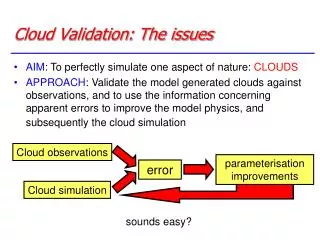
Cloud observations parameterisation improvements error Cloud simulation Cloud Validation: The issues • AIM: To perfectly simulate one aspect of nature: CLOUDS • APPROACH: Validate the model generated clouds against observations, and to use the information concerning apparent errors to improve the model physics, and subsequently the cloud simulation sounds easy?
Cloud Validation: The problems • How much of the ‘error’ derives from observations? Cloud observations error = e1 parameterisation improvements error Cloud simulation error = e2
turbulence radiation cloud physics dynamics convection Cloud Validation: The problems • Which Physics is responsible for the error? Cloud observations parameterisation improvements error Cloud simulation
The path to improved cloud parameterisation… parameterisation improvement ? Composite studies NWP validation Case studies cloud validation Comparison to Satellite Products
Model climate - Broadband radiative fluxes Can compare Top of Atmosphere (TOA) radiative fluxes with satellite observations: TOA Shortwave radiation (TSR) JJA 87 TSR CY18R6-ERBE Stratocumulus regions bad - also North Africa (old cycle!)
Model climate - Cloud radiative “forcing” • Problem: Can we associate these “errors” with clouds? • Another approach is to examine “cloud radiative forcing” JJA 87 SWCRF CY18R6-ERBE Cloud Problems: strato-cu YES, North Africa NO! Note CRF sometimes defined as Fclr-F, also differences in model calculation
Model climate - “Cloud fraction” or “Total cloud cover” Can also compare other variables to derived products: CC JJA 87 TCC CY18R6-ISCCP references: ISCCP Rossow and Schiffer, Bull Am Met Soc. 91, ERBE Ramanathan et al. Science 89
Another approach is to simulate irradiances using model fields Vapour 1 Liquid cloud 1 Ice cloud 1 Radiative transfer model Vapour 2 Liquid cloud 2 Ice cloud 2 Vapour 3 Liquid cloud 3 Ice cloud 3 Height Climatology: The Problems If more complicated cloud parameters are desired (e.g. vertical structure) then retrieval can be ambiguous Channel 1 Channel 2 ….. Assumptions about vertical structures
Examples: Morcrette MWR 1991 Chevallier et al, J Clim. 2001 Simulating Satellite Channels More certainty in the diagnosis of the existence of a problem. Doesn’t necessarily help identify the origin of the problem
DIURNAL CYCLE OVER TROPICAL LAND VARIABILITY A more complicated analysis is possible: Observations: late afternoon peak in convection Model: morning peak (Common problem)
NWP forecast evaluation • Differences in longer simulations may not be the direct result of the cloud scheme • Interaction with radiation, dynamics etc. • E.g: poor stratocumulus regions • Using short-term NWP or analysis restricts this and allows one to concentrate on the cloud scheme Introduction of Tiedtke Scheme cloud cover bias Time
Example over Europe -8:-3 -3:-1 -1:1 1:3 3:8 • What are your conclusions concerning the cloud scheme?
Example over Europe -8:-3 -3:-1 -1:1 1:3 3:8 • Who wants to be a Meteorologist? • Which of the following is a drawback of SYNOP observations? (a) They are only available over land (b) They are only available during daytime (c) They do not provide information concerning vertical structure (d) They are made by people
Case Studies • These were examples of general statistics: globally or for specific regions • Can look concentrate on a particular location in more details, for which more data is collected:CASE STUDY • Examples: • GATE, CEPEX, TOGA-COARE, ARM...
Evaluation of vertical cloud structure Mace et al., 1998, GRL Examined the frequency of occurrence of ice cloud Reasonable match to data found ARM Site - America Great Plains
Evaluation of vertical cloud structure Hogan et al., 2000, JAM Analysis using the Chilbolton radar and Lidar Reasonable Match
Hogan et al. Found that comparison improved when snow was taken into account
Issues Raised: • WHAT ARE WE COMPARING? • Is the model statistic really equivalent to what the instrument measures? • e.g: Radar sees snow, but the model may not include this is the definition of cloud fraction. Small ice amounts may be invisible to the instrument but included in the model statistic • HOW STRINGENT IS OUR TEST? • Perhaps the variable is easy to reproduce • e.g: Mid-latitude frontal clouds are strongly dynamically forced, cloud fraction is often zero or one. Perhaps cloud fraction statistics are easy to reproduce in short term forecasts
Can also use to validate “components” of cloud scheme EXAMPLE: Cloud Overlap Assumptions Hogan and Illingworth, 00, QJRMS Issues Raised: HOW REPRESENTATIVE IS OUR CASE STUDY LOCATION? e.g: Wind shear and dynamics very different between Southern England and the tropics!!!
Composites • We want to look at a certain kind of model system: • Stratocumulus regions • Extra tropical cyclones • An individual case may not be conclusive: Is it typical? • On the other hand general statistics may swamp this kind of system • Can use compositing technique
120 120 250 250 1. 2. 350 350 500 500 620 620 750 750 900 900 Composites - a cloud survey From Satellite attempt to derive cloud top pressure and cloud optical thickness for each pixel - Data is then divided into regimes according to sea level pressure anomaly Use ISCCP simulator Data Model Modal-Data -ve SLP Tselioudis et al., 2000, JCL Cloud top pressure +ve SLP • High Clouds too thin • Low clouds too thick Optical depth
Composites – Extra-tropical cyclones Overlay about 1000 cyclones, defined about a location of maximum optical thickness Plot predominant cloud types by looking at anomalies from 5-day average • High Clouds too thin • Low clouds too thick High tops=Red, Mid tops=Yellow, Low tops=Blue Klein and Jakob, 1999, MWR
A strategy for cloud parametrization evaluation Jakob, Thesis Where are the difficulties?
Recap: The problems • All Observations • Are we comparing ‘like with like’? What assumptions are contained in retrievals/variational approaches? • Long term climatologies: • Which physics is responsible for the errors? • Dynamical regimes can diverge • NWP, Reanalysis, Column Models • Doesn’t allow the interaction between physics to be represented • Case studies • Are they representative? Do changes translate into global skill? • CompositesAs case studies. • And one more problem specific to NWP…
NWP cloud scheme development Timescale of validation exercise • Many of the above validation exercises are complex and involved • Often the results are available O(years) after the project starts for a single version of the model • NWP operational models are updated 2 to 4 times a year roughly, so often the validation results are no longer relevant, once they become available. Requirement: A quick and easy test bench
26r1: April 2003 Example: LWP ERA-40 and recent cycles model 23r4: June 2001 SSMI Diff
Example: LWP ERA-40 and recent cycles model 23r4: June 2001 26r3: Oct 2003 SSMI Diff
Example: LWP ERA-40 and recent cycles model 23r4: June 2001 28r1: Mar 2004 SSMI Diff
Example: LWP ERA-40 and recent cycles model 23r4: June 2001 28r3: Sept 2004 SSMI Diff
Example: LWP ERA-40 and recent cycles model 23r4: June 2001 29r1: Apr 2005 SSMI Diff Do ERA-40 cloud studies still have relevance for the operational model?
So what is used at ECMWF? • T799-L91 • Standard “Scores” (rms, anom corr of U, T, Z) • “operational” validation of clouds against SYNOP observations • Simulated radiances against Meteosat 7 • T159-L91 – “climate” runs • 3 ensemble members of 13 months • Automatically produces comparisons to: • ERBE, NOAA-x, CERES TOA fluxes • Quikscat & SSM/I, 10m winds • ISCCP & MODIS cloud cover • SSM/I, TRMM liquid water path • (soon MLS ice water content) • GPCP, TRMM, SSM/I, Xie Arkin, Precip • Dasilva climatology of surface fluxes • ERA-40 analysis winds All datasets treated as “truth”
OLR -150 Model T95 L91 -300 -150 CERES Conclusions? -300 too high Difference too low
SW 350 Model T95 L91 100 350 CERES Conclusions? 100 albedo high Difference albedo low
TCC 80 Model T95 L91 5 80 ISCCP Conclusions? 5 TCC high Difference TCC low
First Ice Validation: microwave limb sounders 316 hPa 215 hPa Color: MLS White bars: EC IWC sampled with MLS tracks
TCLW LWP 80 Model T95 L91 5 80 SSMI Conclusions? 5 high Difference low
Daily Report 11th April 2005Lets see what you think? “Going more into details of the cyclone, it can be seen that the model was able to reproduce the very peculiar spiral structure in the clouds bands. However large differences can be noticed further east, in the warm sector of the frontal system attached to the cyclone, were the model largely underpredicts the typical high-cloud shield. Look for example in the two maps below where a clear deficiency of clod cover is evident in the model generated satellite images north of the Black Sea. In this case this was systematic over different forecasts.” – Quote from ECMWF daily report 11th April 2005
Same Case, water vapour channels Blue: moist Red: Dry 30 hr forecast too dry in front region Is not a FC-drift, does this mean the cloud scheme is at fault?
Future: Long term ground-based validation, CLOUDNET • Network of stations processed for multi-year period using identical algorithms, first Europe, now also ARM sites • Some European provide operational forecasts so that direct comparisons are made quasi-realtime • Direct involvement of Met services to provide up-to-date information on model cycles
Cloudnet Example • In addition to standard quicklooks, longer-term statistics are available • This example is for ECMWF cloud cover during June 2005 • Includes preprocessing to account for radar attenuation and snow • See www.cloud-net.org for more details and examples!
Future: Improved remote sensing capabilities, CLOUDSAT • CloudSat is an experimental satellite that will use radar to study clouds and precipitation from space. CloudSat will fly in orbital formation as part of the A-Train constellation of satellites (Aqua, CloudSat, CALIPSO, PARASOL, and Aura) • Launched 28th April
Cloudsat transect Zonal mean cloud cover
A chasm still exists!!! cloud validation In summary: Many methods for examining clouds but all too often... parameterisation improvement