Download

1 / 24
240 likes | 342 Views
Explore problems that cannot be efficiently solved in computational theory, P vs. NP, Finite Automata Languages, Turing Machines, Decision Versions, Time and Space Complexity Classes, and more. Understand the boundaries of computability and various computational models. Discover key concepts in the theory of computing.

E N D
Theory of Computing Lecture 15 MAS 714 Hartmut Klauck
Part II Overview • Problems that cannot be solved efficiently • P vs. NP • Time Hierarchy • Problems that cannot be solved at all • Computability • Weaker models of computation • Finite Automata
Languages • Definition: • An alphabet is a finite set of symbols • ¡* is the set of all finite sequences/strings over the alphabet ¡ • A language over alphabet ¡ is a subset of ¡* • A machine decides a language L if on input x it outputs 1 if x2L and 0 otherwise • A complexity class is a set of languages that can be computed given some restricted resources
The Class P • The class P consists of all languages that can be decided in polynomial time • Which machine model? • RAM’s with the logarithmic cost measure • Simpler: Turing machines • Polynomial size circuits (with simple descriptions)
The Class P • For technical reasons P contains only decision problems • Example: Sorting can be done in polynomial time, but is not a language • Decision version: • ElementDistinctness={x1,…, xn: the xi are pairwise distinct} • ElementDistinctness2P
The Class P • Problems solvable in polynomial time? • Sorting • Minimum Spanning Trees • Matching • Max Flow • Shortest Path • Linear Programming • Many more • Decision version example: {G,W,K: there is a spanning tree of weight at most K in G}
Turing Machine • Defined by Turing in 1936 to formalize the notion of computation • A Turing machine has a finite control and a 1-dimensional storage tape it can access with its read/write head • Operation: the machine reads a symbol from the tape, does an internal computation and writes another symbol to the tape, moves the head
Turing Machine • A Turing machine is a 8-tuple(Q, ¡, b, §, q0, A,R, ±) • Q: set of states of the machine • ¡: tape alphabet • b2¡: blank symbol • §µ¡-{b}: input alphabet • q02 Q: initial state • A,R µ Q: accepting/rejecting states • ±: Q- (A[R) £¡ Q£¡£{left,stay,right}: transition function
Operation • The tape consists of an infinite number of cells labeled by all integers • In the beginning the tape contains the input x2§* starting at tape cell 0 • The rest of the tape contains blank symbols • The machine starts in state q0 • The head is on cell 0 in the beginning
Operation • In every step the machine reads the symbol z at the position of the head • Given z and the current state q it uses ± to determine the new state, the symbol that is written to the tape and the movement of the head • left, stay, right • If the machine reaches a state in A it stops and accepts, on states in R it rejects
Example Turing Machine • To compute the parity of x2{0,1}* • Q={q0, q1, qa, qr} • ¡={0,1,b} • ±:q0 ,1 q1,b, rightq0,0 q0,b, rightq1,1 q0,b, rightq1,0 q1,b, rightq1, b qaq0,b qr
Example • The Turing machine here only moves right and does not write anything useful • It is a finite automaton
Correctness/Time • A TM decides L if it accepts all x2L and rejects all x not in L (and halts on all inputs) • The time used by a TM on input x is the number of steps [evaluations of ±] before the machine reaches a state in A or R • The time complexity of a TM M is the function tM that maps n to the largest time used on any input in ¡ n • The time complexity of L is upper bounded by g(n) if there is a TM M that decides L and has tM(n)·O(g(n))
Notes • DTIME(f(n)) is the class of all languages that have time complexity at most O(f(n)) • P is the class of languages L such that the time complexity of L can be upper bounded by a fixed polynomial in n [with a fixed highest power of n appearing in p] • There are languages for which there is no asymptotically fastest TM [Speedup theorem]
Space • The space used by a TM M on an input x is the number of cells visited by the head • The space complexity of M is the function sM mapping n to the largest space used on x2¡ n • The space complexity of L is upper bounded by g(n) if there is a TM that decides L and sM(n)=O(g(n))
Facts • A Turing machine can simulate a RAM with log cost measure such that • polynomial time RAM gives a polynomial time TM • A log-cost RAM can simulate a TM • Store the tape in the registers • Store the current state in a register • Each register stores a symbol or state [O(1) bits] • Store also the head position in a register [log sM bits] • Compute the transition function by table lookup • Hence the definition of P is robust
Criticism • P is supposed to represent efficiently solvable problems • P contains only languages • Can identify a problem with many outputs with a set of languages (one for each output bit) • Problems with time complexity n1000 are deemed easy while problems with time complexity 2n/100000 hard • Answer: P is mainly a theoretical tool • In practice such problems don’t seem to arise • Once a problem is known to be in P we can start searching for more efficient algorithms
Criticism • Turing machines might not be the most powerful model of computation • All computers currently built can be simulated efficiently • Small issue: randomization • Some models have been proposed that are faster, e.g. analogue computation • Usually not realistic models • Exception: Quantum computers • Quantum Turing machines are probably faster than Turing machines for some problems
Why P? • P has nice closure properties • Example: closed under calling subroutines: • Suppose R2P • If there is a polynomial time algorithm that solves L given a free subroutine that computes R, then L is also in P
Variants of TM • Several tapes • Often easier to describe algorithms • Example: Palindrome={xy: x is y in reverse} • Compute length, copy x on another tape, compare x and y in reverse • Any 1-tape TM needs quadratic time • Any TM with O(1) tapes and time T(n) can be simulated by a 1-tape TM using time T(n)2
Problems that are not in P • EXP: class of all L that can be decided by Turing machines that run in time at most exp(p(n)) for some polynomial p • We will show later that EXP is not equal to P • i.e., there are problems that can be solved in exponential time, but not in polynomial time • These problems tend to be less interesting
Problems that are not in P? • Definition: • Given an undirected graph, a clique is a set of vertices Sµ V, such that all u,v2 S are connected • The language MaxClique is the set of all G,k, such that G has a clique of size k (or more) • Simple Algorithm: enumerate all subsets of size k, test if they form a clique • Time O(nk¢ poly(k)) • Since k is not constant this is not a polynomial time algorithm
Clique • It turns out that MaxClique is in P if and only if thousands of other interesting problems are • We don’t know an efficient algorithm for any of them • Widely believed: there is no such algorithm
Fun Piece of Information • A random graph is a graph generated by putting each possible edge into G with probability ½ • The largest clique in G has size dr(n)e or br(n)cfor an explicit r(n) that is around (2+o(1)) log(n) • with probability approaching 1 • Hence on random graphs the max clique can be found in sub-exponential time