Download

1 / 0
10 likes | 129 Views
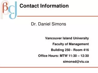
Reach out to Dr. Daniel Simons at Vancouver Island University's Faculty of Management for academic guidance. Located in Building 250, Room 416, Dr. Simons is available for consultations during office hours on Mondays, Wednesdays, and Fridays from 12:00 PM to 1:00 PM. For optimal individual performance, it is suggested that students attend all classes to enhance learning and engagement. Connect at simonsd@viu.ca for any inquiries or support.

E N D