Download

1 / 19
200 likes | 212 Views
Taming the Curse of Dimensionality: Discrete Integration by Hashing and Optimization. Stefano Ermon* , Carla P. Gomes*, Ashish Sabharwal + , and Bart Selman* *Cornell University + IBM Watson Research Center ICML - 2013. High-dimensional integration.

E N D
Taming the Curse of Dimensionality: Discrete Integration by Hashing and Optimization Stefano Ermon*, Carla P. Gomes*, Ashish Sabharwal+, and Bart Selman* *Cornell University +IBM Watson Research Center ICML - 2013
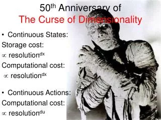
High-dimensional integration • High-dimensional integrals in statistics, ML, physics • Expectations / model averaging • Marginalization • Partition function / rank models / parameter learning • Curse of dimensionality: • Quadrature involves weighted sum over exponential number of items (e.g., units of volume) n dimensional hypercube L2 L3 L4 Ln L
Discrete Integration Size visually represents weight 2n Items 5 • We are given • A set of 2n items • Non-negative weights w • Goal: compute total weight • Compactly specified weight function: • factored form (Bayes net, factor graph, CNF, …) • potentially Turing Machine • Example 1: n=2 dimensions, sum over 4 items • Example 2: n= 100 dimensions, sum over 2100 ≈1030 items (intractable) 4 1 … 0 5 1 0 2 5 2 Goal: compute 5 + 0 + 2 + 1 = 8 1 0
Hard EXP Hardness PSPACE P^#P PH 0 1 • 0/1 weights case: • Is there at least a “1”? SAT • How many “1” ? #SAT • NP-complete vs. #P-complete. Much harder • General weights: • Find heaviest item (combinatorial optimization) • Sum weights (discrete integration) • This Work: Approximate Discrete Integration via Optimization • Combinatorial optimization (MIP, Max-SAT,CP) also often fast in practice: • Relaxations / bounds • Pruning NP P 0 1 Easy 0 3 4 7
Previous approaches: Sampling Idea: • Randomly select a region • Count within this region • Scale up appropriately Advantage: • Quite fast Drawback: • Robustness: can easily under- or over-estimate • Scalability in sparse spaces:e.g. 1060 items with non-zero weight out of 10300 means need region much larger than 10240 to “hit” one • Can be partially mitigated using importance sampling 60 9 5 2 70 5 5 2 100 5 5 5 9 9 2 5
Previous approaches: Variational methods Idea: • For exponential families, use convexity • Variational formulation (optimization) • Solve approximately (using message-passing techniques) Advantage: • Quite fast Drawback: • Objective function is defined indirectly • Cannot represent the domain of optimization compactly • Need to be approximated (BP, MF) • Typically no guarantees
A new approach : WISH 2i-largest weight (quantile) bi Suppose items are sorted by weight b4=2 b3=5 b1=70 b0=100 b2=9 100 70 60 9 9 9 5 5 5 5 5 5 5 2 2 2 Geometrically increasing bin sizes 8 4 2 1 1 CDF-style plot Area under the curve equals the total weight we want to compute. How many items with weight at least b # items How to estimate? Divide into slices and sum up 1 w Geometrically divide y axis Given the endpoints bi, we have a 2-approximation Can bound area in each slice within a factor of 2 Also works if we have approximations Mi of bi b How to estimate the bi?
Estimating the endpoints (quantiles) bi Hash 2n items into 2i buckets, then look at a single bucket. Find heaviest weight wi in the bucket. For i=2, hashing 16 items into 22=4 buckets 9 5 70 2 5 5 9 2 5 9 100 5 60 5 5 2 Wi=9 INTUITION. Repeat several times. With High Probability: wi oftenfound to be larger than w*there are at least 2i items with weight larger than w*.
Hashing and Optimization • Hash into 2i buckets, then look at a single bucket • With probability >0.5: • There is nothing from the small set (vanishes) • There is something from the larger set (survives) 2 5 9 2i-2=2i/4 heaviest items 100 5 bi-2 bi+2 b0 bi 16 times larger Geometrically increasing bin sizes increasing weight 100 2i+2=4.2i heaviest items 2 Remember items are sorted so max picks the “rightmost” item… Something in here is likely to be in the bucket, so if we take a max , it will be in this range
Universal Hashing Bucket content is implicitly defined by the solutions of A x = b mod 2 (parity constraints) • Represent each item as an n-bit vector x • Randomly generate A in {0,1}i×n,b in {0,1}i • Then A x + b (mod 2) is: • Uniform • Pairwise independent n A x b i = (mod 2) bi+2 bi-2 b0 bi x x x x x Max w(x) subject to A x = b mod 2 is in here “frequently” Repeat several times. Median is in the desired range with high probability
WISH : Integration by Hashing and Optimization WISH (WeightedIntegralsSumsByHashing) • T = log (n/δ) • For i = 0, … , n • For t = 1, … ,T • Sample uniformly A in {0,1}i×n, b in {0,1}i • wit = max w(x) subject to A x = b (mod 2) • Mi = Median (wi1, … , wiT) • Return M0 + Σi Mi+1 2i The algorithm requires only O(n log n) optimizations for a sum over 2n items Outer Loop over n+1 endpoints of the n slices (bi) Hash into 2i buckets Find heaviest item Repeat log(n) times CDF-style plot Mi estimates the 2i-largest weight bi Sum up estimated area in each vertical slice # items
Visual working of the algorithm n times • How it works 1 random parity constraint 2 random parity constraints 3 random parity constraints Function to be integrated …. …. …. …. Log(n) times Mode M0 + median M1 + median M2 + median M3 ×4 ×1 ×2 + …
Accuracy Guarantees • Theorem 1: With probability at least 1- δ (e.g., 99.9%) WISH computes a 16-approximation of a sum over 2n items (discrete integral) by solving θ(n log n) optimization instances. • Example: partition function by solving θ(n log n) MAP queries • Theorem 2: Can improve the approximation factor to (1+ε) by adding extra variables. • Example: factor 2 approximation with 4n variables • Byproduct: we also obtain a 8-approximation of the tail distribution (CDF) with high probability
Key features • Strong accuracy guarantees • Can plug in any combinatorial optimization tool • Bounds on the optimization translate to bounds on the sum • Stop early and get a lower bound (anytime) • (LP,SDP) relaxations give upper bounds • Extra constraints can make the optimization harder or easier • Massively parallel (independent optimizations) • Remark: faster than enumeration force only when combinatorial optimization is efficient (faster than brute force).
Experimental results • Approximate the partition function of undirected graphical models by solving MAP queries (find most likely state) • Normalization constant to evaluate probability, rank models • MAP inference on graphical model augmented with random parity constraints • Toulbar2 (branch&bound) solver for MAP inference • Augmented with Gauss-Jordan filtering to efficiently handle the parity constraints (linear equations over a field) • Run in parallel using > 600 cores Parity check nodes enforcing A x = b (mod 2) Original graphical model
Sudoku • How many ways to fill a valid sudoku square? • Sum over 981 ~ 1077 possible squares (items) • w(x)=1 if it is a valid square, w(x)=0 otherwise • Accurate solution within seconds: • 1.634×10²¹ vs 6.671×10²¹ …. ? 1 2
Random Cliques Ising Models Very small error band is the 16-approximation range Strength of the interactions Other methods fall way out of the error band Partition function MAP query
Model ranking - MNSIT • Use the function estimate to rank models (data likelihood) • WISH ranks them correctly. Mean-field and BP do not. Visually, a better model for handwritten digits
Conclusions • Discrete integration reduced to small number of optimization instances • Strong (probabilistic) accuracy guarantees by universal hashing • Can leverage fast combinatorial optimization packages • Works well in practice • Future work: • Extension to continuous integrals • Further approximations in the optimization [UAI -13] • Coding theory / Parity check codes / Max-Likelihood Decoding • LP relaxations • Sampling from high-dimensional probability distributions?