Download
1 / 44
470 likes | 505 Views
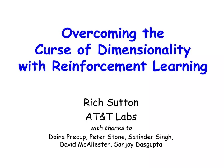
Overcoming the Curse of Dimensionality with Reinforcement Learning. Rich Sutton AT&T Labs with thanks to Doina Precup, Peter Stone, Satinder Singh, David McAllester, Sanjoy Dasgupta. Computers have gotten faster and bigger. Analytic solutions are less important

E N D
Overcoming theCurse of Dimensionality with Reinforcement Learning Rich Sutton AT&T Labs with thanks to Doina Precup, Peter Stone, Satinder Singh, David McAllester, Sanjoy Dasgupta
Computers have gotten faster and bigger • Analytic solutions are less important • Computer-based approximate solutions • Neural networks • Genetic algorithms • Machines take on more of the work • More general solutions to more general problems • Non-linear systems • Stochastic systems • Larger systems • Exponential methods are still exponential… but compute-intensive methods increasingly winning
New Computers have led to aNew Artificial Intelligence More general problems and algorithms, automation - Data intensive methods - learning methods Less handcrafted solutions, expert systems More probability, numbers Less logic, symbols, human understandability More real-time decision-making States, Actions, Goals, Probability => Markov Decision Processes
Markov Decision Processes State SpaceS(finite) Action SpaceA(finite) Discrete timet = 0,1,2,… Episode Transition Probabilities Expected Rewards Policy Return Value Optimal policy (discount rate) PREDICTION Problem CONTROL Problem
Key Distinctions • Control vs Prediction • Bootstrapping/Truncation vs Full Returns • Sampling vs Enumeration • Function approximation vs Table lookup • Off-policy vs On-policy Easier, conceptually simpler Harder, more challenging and interesting
Full Depth Search ˆ Computing V(s) s Full Returns 2 L r r r + g ¢ + g ¢ ¢ + a r s’ a’ r’ r” depth BD is of exponential complexity branching factor
Truncated Search Computing V(s) s Truncated Returns ˆ r + g V ( s ) ¢ a r s’ ˆ V ( s ) ¢ Search truncated after one ply Approximate values used at stubs Values computed from their own estimates! -- “Bootstrapping”
ˆ ˆ ˆ V V V Dynamic Programming is Bootstrapping s Truncated Returns ˆ E r V ( s ) s + g ¢ a r s’ ˆ V E.g., DP Policy Evaluation
Bootstrapping/Truncation • Replacing possible futures with estimates of value • Can reduce computation and variance • A powerful idea, but • Requires stored estimates of value for each state
Bellman, 1961 The Curse of Dimensionality • The number of states grows exponentially with dimensionality -- the number of state variables • Thus, on large problems, • Can’t complete even one sweep of DP • Can’t enumerate states, need sampling! • Can’t store separate values for each state • Can’t store values in tables, need function approximation! DP Policy Evaluation
DP Policy Evaluation å å a [ a ] ˆ ˆ V ( s ) ( s , a ) p r V ( s ) s S ¬ p + g ¢ " Î k 1 s s s s k + ¢ ¢ a s ¢ å å a [ a ] ˆ ˆ s S V ( s ) d ( s ) ( s , a ) p r V ( s ) " Î ¬ p + g ¢ k 1 s s s s k + ¢ ¢ a s ¢ Some distribution over states, possibly uniform TD(l) samples the possibilities rather than enumerating and explicitly considering all of them
DP Policy Evaluation å å a [ a ] ˆ ˆ V ( s ) ( s , a ) p r V ( s ) s S ¬ p + g ¢ " Î k 1 s s s s k + ¢ ¢ a s ¢ å å a [ a ] ˆ ˆ s S V ( s ) d ( s ) ( s , a ) p r V ( s ) " Î ¬ p + g ¢ k 1 s s s s k + ¢ ¢ a s ¢ These terms can be replaced by sampling
Sampling vs Enumeration DP Policy Evaluation å å a [ a ] ˆ ˆ V ( s ) ( s , a ) p r V ( s ) s S ¬ p + g ¢ " Î k 1 s s s s k + ¢ ¢ a s ¢ å å a [ a ] ˆ ˆ s S V ( s ) d ( s ) ( s , a ) p r V ( s ) " Î ¬ p + g ¢ k 1 s s s s k + ¢ ¢ a s ¢ Tabular TD(0) Sutton, 1988; Witten, 1974 For each sample transition, s,as’,r :
Sample Returns can also be either Full or Truncated r ˆ r + g V ( s ) ¢ r ¢ As in the general TD(l) algorithm r ¢ ¢ 2 L r r r + g ¢ + g ¢ ¢ +
Function Approximation • Store values as a parameterized form • Update q, e.g., by gradient descent: cf. DP Policy Evaluation (rewritten to include a step-size a):
Linear Function Approximation Each state s represented by a feature vector Or respresent a state-action pair with and approximate action values:
Linear TD(l) After each episode: where T e.g., r + g q f t 1 s a + t + 1 t + 1 “ l-return” “n-step return” Sutton, 1988
RoboCup An international AI and Robotics research initiative • Use soccer as a rich and realistic testbed • Robotic and simulation leagues • Open source simulator (Noda) Research Challenges • Multiple teammates with a common goal • Multiple adversaries – not known in advance • Real-time decision making necessary • Noisy sensors and actuators • Enormous state space, > 2310 states 9
RoboCup Feature Vectors . . . Full soccer state . action values . Linear map q Sparse, coarse, tile coding . . . . . 13 continuous state variables . r Huge binary feature vector (about 400 1’s and 40,000 0’s) f s
13 Continuous State Variables(for 3 vs 2) 11 distances among the players, ball, and the center of the field 2 angles to takers along passing lanes
Sparse, Coarse, Tile-Coding (CMACs) 32 tilings per group of state variables
Learning Keepaway Results3v2 handcrafted takers Multiple, independent runs of TD(l) Stone & Sutton, 2001
Key Distinctions • Control vs Prediction • Bootstrapping/Truncation vs Full Returns • Function approximation vs Table lookup • Sampling vs Enumeration • Off-policy vs On-policy • The distribution d(s)
Off-Policy Instability • Examples of diverging qk are known for • Linear FA • Bootstrapping • Even for • Prediction • Enumeration • Uniform d(s) • In particular, linear Q-learning can diverge Baird, 1995 Gordon, 1995 Bertsekas & Tsitsiklis, 1996
Baird’s Counterexample Markov chain (no actions) All states updated equally often, synchronously Exact solution exists: q= 0 Initial q0 = (1,1,1,1,1,10,1)T 100% ±1)
On-Policy Stability • If d(s) is thestationary distribution of the MDP under policy p (the on-policy distribution) • Then convergence is guaranteed for • Linear FA • Bootstrapping • Sampling • Prediction • Furthermore, asymptotic mean square error is a bounded expansion of the minimal MSE: Tsitsiklis & Van Roy, 1997 Tadic, 2000
V* — Value Function Space — True V* best admissable value fn. Region of * Original naïve hope inadmissable value functions guaranteed convergence to good policy best admissable policy value functions consistent with parameterization Sarsa, TD(l) & other on-policy methods Res gradient et al. chattering without divergence or guaranteed convergence Q-learning, DP & other off-policy methods guaranteed convergence to less desirable policy divergence possible
There are Two Different Problems: • Chattering • Is due to Control + FA • Bootstrapping not involved • Not necessarily a problem • Being addressed with • policy-based methods • Argmax-ing is to blame • Instability • Is due to Bootstrapping • + FA + Off-Policy • Control not involved • Off-policy is to blame
Yet we need Off-policy Learning • Off-policy learning is needed in all the frameworks that have been proposed to raise reinforcement learning to a higher level • Macro-actions, options, HAMs, MAXQ • Temporal abstraction, hierarchy, modularity • Subgoals, goal-and-action-oriented perception • The key idea is: We can only follow one policy, but we would like to learn about many policies, in parallel • To do this requires off-policy learning
On-Policy Policy Evaluation Problem Use data (episodes) generated by p to learn Off-Policy Policy Evaluation Problem Use data (episodes) generated by p’ to learn Target policy behavior policy
Naïve Importance-Sampled TD(l) Relative prob. of episode under p and p’ r r r r L 1 2 3 T-1 importance sampling correction ratio for t We expect this to have relatively high variance
is like , except in terms of Per-Decision Importance-Sampled TD(l) L r r r r 1 2 3 t
Per-Decision TheoremPrecup, Sutton & Singh (2000) New Result for Linear PD AlgorithmPrecup, Sutton & Dasgupta (2001) Total change over episode for new algorithm Total change for conventional TD(l)
Convergence Theorem • Under natural assumptions • S and A are finite • All s,a are visited under p’ • p and p’ are proper (terminate w.p.1) • bounded rewards • usual stochastic approximation conditions on the step size ak • And one annoying assumption • Then the off-policy linear PD algorithm converges to the same qas on-policy TD(l) e.g., bounded episode length
The variance assumption is restrictive But can often be satisfied with “artificial” terminations • Consider a modified MDP with bounded episode length • We have data for this MDP • Our result assures good convergence for this • This solution can be made close to the sol’n to original problem • By choosing episode bound long relative to g or the mixing time • Consider application to macro-actions • Here it is the macro-action that terminates • Termination is artificial, real process is unaffected • Yet all results directly apply to learning about macro-actions • We can choose macro-action termination to satisfy the variance condition
Empirical Illustration Agent always starts at S Terminal states marked G Deterministic actions Behavior policy chooses up-down with 0.4-0.1 prob. Target policy chooses up-down with 0.1-0.4 If the algorithm is successful, it should give positive weight to rightmost feature, negative to the leftmost one
Trajectories of Two Components of q 0 . 5 0 . 4 0 . 3 * µ r i g h t m o s t , d o w n 0 . 2 µ l = 0.9 a decreased 0 . 1 r i g h t m o s t , d o w n 0 - 0 . 1 µ l e f t m o s t , d o w n * - 0 . 2 µ l e f t m o s t , d o w n - 0 . 3 - 0 . 4 0 1 2 3 4 5 E p i s o d e s x 1 0 0 , 0 0 0 q appears to converge as advertised
Comparison of Naïve and PD IS Algs 2 . 5 l = 0.9 a constant N a i v e I S R o o t M e a n 2 S q u a r e d E r r o r Per-Decision IS 1 . 5 (after 100,000 episodes, averaged over 50 runs) 1 - 1 2 - 1 3 - 1 4 - 1 5 - 1 6 - 1 7 Log2 a Precup, Sutton & Dasgupta, 2001
ith return following s,a IS correction product L r r r r t 1 t 2 t 3 T 1 + + + - (s,a occurs at t ) Can Weighted IS help the variance? Return to the tabular case, consider two estimators: converges with finite variance iff the wi have finite variance Can this be extended to the FA case? converges with finite variance even if the wi have infinite variance
Restarting within an Episode • We can consider episodes to start at any time • This alters the weighting of states, • But we still converge, • And to near the best answer (for the new weighting)
Incremental Implementation At the start of each episode: On each step:
Key Distinctions • Control vs Prediction • Bootstrapping/Truncation vs Full Returns • Sampling vs Enumeration • Function approximation vs Table lookup • Off-policy vs On-policy Easier, conceptually simpler Harder, more challenging and interesting
Conclusions • RL is beating the Curse of Dimensionality • FA and Sampling • There is a broad frontier, with many open questions • MDPs: States, Decisions, Goals, and Probability is a rich area for mathematics and experimentation