Download

1 / 46
610 likes | 1.12k Views
Travelling Salesman Problem (TSP). Aayush Singhal (09005041) Gaurav Torka (09005051) Sai Teja Pratap (09005057) Guide: Prof Pushpak Bhattacharyya. Introduction. Definition:

E N D
Travelling Salesman Problem (TSP) AayushSinghal (09005041) GauravTorka(09005051) SaiTejaPratap (09005057) Guide: Prof Pushpak Bhattacharyya
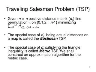
Introduction Definition: Given a set of cities and the distance between each possible pair, the Travelling Salesman Problem is to find the best possible way of ‘visiting all the cities exactly once and returning to the starting point’
A Brief History • The problem was first defined in the 1800s by the Irish mathematician W.R. Hamilton and the British mathematician Thomas Kirkman. • It was, however, first formulated as a mathematical problem only in 1930 by Karl Menger. • The name Travelling Salesman Problem was introduced by American HasslerWhiteney. • The origin of TSP lies with Hamilton's Icosian Game, which was a recreational puzzle based on finding a Hamiltonian cycle. • Richard M. Karp showed in 1972 that the Hamiltonian cycle problem was NP-complete, which implies the NP-hardness of TSP. This supplied a mathematical explanation for the apparent computational difficulty of finding optimal tours.
TSP : An NP-HARD Problem! • TSP is an NP-hard problem in combinatorial optimization studied in theoretical computer science. • In many applications, additional constraints such as limited resources or time windows make the problem considerably harder. • Removing the constraint of visiting each city exactly one time also doesn't reduce complexity of the problem. • In spite of the computational difficulty of the problem, a large number of heuristics and exact methods are known, which can solve instances with thousands of cities.
Applications of TSP • Even in its purest form the TSP, has several applications such as planning, logistics, and the manufacture of microchips. • Slightly modified, it appears as a sub-problem in many areas, such as DNA sequencing. • In these applications, the concept city represents, for example, customers, soldering points, or DNA fragments • The concept distance represents travelling times or cost, or a similarity measure between DNA fragments. • As TSP is a NP hard problem it is often used as a benchmark for optimization techniques.
Applications of TSP Mechanical arm • When a mechanical arm is used to fasten the nuts for assembling parts, it moves through each nut in proper order and returns to the initial position. • The most economical travelling route will enable the mechanical arm to finish its work within the shortest time. Integrated circuit • Inserting electrical elements in the manufacturing of integrated circuits consumes certain energy when moving from one electrical element to the other during manufacturing. • We need to arrange the manufacturing order to minimize the energy consumption. In both these cases, TSP is required to be solved as a sub-problem.
Useful Variations of TSP Variations of TSP might be desired in certain real-life scenarios • In transportation-based graphs, the edge weights can change constantly when they are based on the time to traverse the roadway they represent. • It might not be necessary to visit every node in a route, so a route that visits only a predefined subset of nodes needs to be determined. • A node can be visited more than once if that provides a faster route. • Visiting a certain unwanted node might be useful in obtaining a faster route.
Exact Solution • A direct solution is to try out all the permutations and find out the shortest of all these permutations. • This would be O(n!) time complexity, which implies 10^64 for 50 cities. This is practically useless. • Other approaches attempted at solving the problem include Dynamic Programming, branch and bound, linear programming. • None of them were feasible for number of cities over 500. It has not been determined whether an exact algorithm for TSP that runs in O(1.9999^n) time exists. • So attempts have are made to solve TSP approximately which give sub optimal solutions. • Here we present a few intelligent approaches to solve TSP approximately.
Solving TSP using A-star • As A-star is general graph search algorithm it can be used for solving TSP. • As the length of the tour for the best solution is not known the first challenge is to determine the goal of the A-Star search. • With the given configuration one can find the upper and lower bounds for the best solution. • Then do a binary search running A-star each time to check if the given goal length is feasible. • Alternatively one can have terminating condition instead of a goal and run the A-star search until the condition is met.
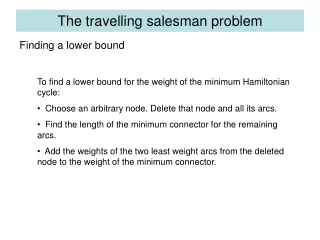
A state is a path in the graph, that visits any node at most once.
Heuristic and State Space • At any point during the execution we have a path formed up till that point of time and a set of vertices which have to be added to the path to complete the tour .This forms the state space . • We represent a state as S(i1 ,i2..ik) which means the path formed so far is i1 ,i2..ik and the remaining vertices are to be added to the tour. • A heuristic can be the weight of MST of the remaining vertices.
How good is this State Space? • Let S(k) denote the set of all states which have a formed a path for k vertices. • Number of elements in S(k) is P(n,k) = (n!/(n-k)!) • So total number of states would be S = P(n,0) + P(n,1) + P(n,2) …… P(n,n-1) + P(n,n) S < n! + n! + n! ……. n! + n! S < (n+1)n! S < (n+1)! • The number of states is of the order of factorial of n But we don’t need to store the state space.
Defining the Edges • The edge weight between two states is given as follows X =S(i1 ,i2..ik) Y1 =S(i0 ,i1, i2,..ik) Wt(X,Y1) = wt(i1, i0) Y2 =S(i1 ,i2..ik+1) Wt(X,Y2) = wt(ik+1, ik) • Wt(A,B) is the weight of the edge A-B in the A-star state space and wt(a,b) is the weight of the edge a-b in the given graph. • ikand i0 should not belong the set {i1 i2 ……….ik} • No other edges exist • Thus for a given state one can find all its neighbors by adding each of the unvisited nodes to the path. • So for each element in S(k) there are 2(n-k) neighbours.
Feasibility • If a goal length is given we can check the feasibility of the goal in the following way. • If there is one element of set S(n) in the open list, then the search is performed for a fixed number of iterations (call it maxIter) from that point of execution. • In each iteration search in the open list for the solution of desired length. • If one such solution is found, then declare that the given length is feasible and terminate the algorithm. • If no such solution is found within the maxIter number of iterations then the given length is declared as not feasible. • This means that one may miss the exact solution depending upon the value of max iterations.
Terminating condition • If there is no fixed goal length given, then the algorithm’s terminating condition will be as follows. • There are n! elements in the set of solutions S(n) (not necessarily the best) • The approach can be running the search until K elements of the set S(n) are in the open list . • Once this condition is met give the best among these K elements is declared as the solution and the algorithm is terminated.
Genetic Algorithms for TSP • Genetic algorithms are a whole new class of Algorithms which mimic nature and evolution. • They follow Darwin's theory of survival of the fittest. • They are randomized algorithms and may not find best solution. • Using Genetic algorithms we can easily solve problems of size less than 100.
Genetic Algorithms for TSP • Genetic algorithm starts with a random population, and generates modern and new population • It replaces the weak candidates by newly formed strong and useful candidates • In TSP, a permutation is a candidate for population of Genetic Algorithms (GA) • Graph can trivially be converted to a completely connected graph, by inserting edges having infinite weight.
Genetic Algorithms for TSP Genetic algorithm has many steps in it • Evolution • finding out good members from the population • Cross Over • combining two parent members to form two new different members(children) with similar characteristics as parents. • Mutation • Some of newly formed members are altered randomly • Keeps them from becoming identical and converging to a local minima
Completing the graph • Missing edges are inserted with a weight of Infinity (INF)
Genetic Algorithms for TSP • Select some random permutations of cities as initial population • Pick some permutations randomly & reproduce in that subset • In a selected subset, replace worst 2 permutations with 2 new generated permutations • Best 2 permutations in subset are made to be parents • Goodness of permutation is inversely related to path length of that permutation • Smaller path length implies better permutation • Process of generating new permutation from 2 old permutations is called cross over
Cross Over Parent 1 - FAB | ECGD Parent 2 - DEA | CGBFCombining first part of parent 1 with 2nd part of parent 2 and vice versa Child1 – FAB CGBF Child2 – DEA ECGD • Children permutations are not valid permutations, Need different crossover algorithm
Cross Over • Instead of considering the permutation, we can only consider the neighbors of each city in permutation • e.g., in FABCEGD, neighbors of A are F and B. • For cities have same pair of neighbors in both parent, will have same pair of neighbors in both children also • Otherwise neighbors of a city will come as first neighbor of that city in one parent and second in other parent and vice versa for other children. • E.g., if neighbors of A are F, B in parent 1 and C, D in parent 2. Then new neighbors of A are F,D and C,B
Mutation • To avoid generating similar kind of children, some permutations are selected randomly, and they are changed little bit. • E.g., In a permutation, we can swap any two cities. • Do we ever stop? • After finite number of generations or • When permutations start becoming very similar
Ant Colony Algorithm (ACA) • This Algorithm is inspired by the social life of ants • Individual ants are un-intelligent and they are practically blind • But with their social structure ants complete the complex task of finding the shortest path without knowing problem’s existence. • How do they achieve this? (Next Page)
ACA - Background • The ants have a place where they store their food (lets call it a nest). • When they sense some food nearby their task is to carry the food to the nest (preferably in the shortest path) • Ants leave behind a chemical substance called pheromone which lets the other ants identify that an ant has been there before. • The amount of pheromone that an ant deposits is inversely proportional to the distance it has travelled. • So the ants that move along smaller paths secrete more amount of pheromone per unit length.
ACA – The Ant’s way • In the colony ,an ant (called blitz) moves randomly around the colony • If it discovers a food source, it returns directly to the nest, leaving in its path a trail of pheromone • These pheromones attract nearby ants which will be inclined to follow the track • Returning to the colony, these ants will strengthen the route they follow.
ACA – The Ant’s way • If there are two routes to reach the same food source then the shorter one will be traveled by more ants than the long route as the pheromone density is high along them • The short route will be increasingly enhanced, and therefore become more attractive; • The long route will eventually disappear as pheromones are volatile • Eventually, all the ants take shortest route.
ACA into TSP • Ants are simple agents which travel from one city to another city. • Each edge has some pheromone quantity associated with it • The pheromone quantities change dynamically with the ants’ motion in the graph • An ant decides to take an edge depending upon the edge length and the pheromone quantity • The pheromone in each edge is decreased by a constant factor with time.
Pseudo Code procedure ACO algorithm for TSPs Set parameters, initialize pheromone trails while (termination condition not met) do ConstructSolutions UpdateTrails end end ACO algorithm for TSPs
ACA into TSP - details • Initially, all the ants are placed at randomly chosen cities. • At each city, the ant probabilistically chooses a city not yet visited , based on pheromone trail strength on the arc and the distance between them . • Each ant has a limited form of memory, called a Tabu list in which the current partial tour is stored.
ACA into TSP - details • The probability that an ant k moves to city-j when at city-i in iteration number t is given by the following relation. • gives the list of feasible neighbors of city-i for the ant k . • The symbol gives the pheromone quantity for a given edge ij in iteration number t. • The symbol gives the inverse of the edge weight for the edge between city-i and city-j.
Pheromone Update • When all the ants have completed a solution, the trail update is done as per the below equations • L gives the tour length of a given ant • One can interpret this as probabilistic version of A-star where there is no coming back if one finds a bad path.
Performance • ACA with some optimizations can give solutions which are very close to the actual solution (less than 1.1 times the actual best solution). • The number of iterations should be 5 to 10 times the number of cities. • The number of ants should be of the order of number of cities. • For number of cities set to 500 the algorithm gives very good results in 4-5 minutes (around 3000 iterations). • As the algorithm is probabilistic one cannot always expect the same performance.
Comparision of ACA and Genetic Algorithmic Approach Oliver30,att48,Eil51 are instances of TSP taken from TSPLIB which is a library of sample instances for the TSP. The last column is the best solution available in TSPLIB ACS: Ant Colony System’s solution, GA: Basic Genetic Algorithm’s solution
Ant colony algorithm gives good solutions very close optimal path but the lack of pheromone in initial stages leads to slower speed of convergence. • Genetic Algorithms have rapid global searching capability, but the feedback of information in the system is not utilized to its fullest extent • This may lead to redundant iterations and inefficient solution. • As the number of cities increase ACA becomes slow GA might not give the optimal paths. • So mixed approach is applied is being tested. Research is going on about how to mix both approaches and make it faster and give optimal paths.
Conclusion • Evolutionary algorithms like ACA, Genetic Algorithms are very successful in solving the TSP. • These techniques with some variation can be applied to most of the NP-hard problems in general NP-hard problems can be modeled as graph problems. • As we have seen in the case of ACA and Genetic Algorithms naturally occurring phenomena can be effectively used to model computer algorithms. • So observe nature. Nature has solution to everything!
References • Russel S. and Norvig P., "Artificial Intelligence: a Modern Approach", Prentice Hall, (1998) • Adaptive Ant Colony Optimization for the Traveling Salesman Problem, Michael Maur(2009 ) • An Ant Colony Optimization Algorithm for the Stable Roommates Problem Glen Upton(2002) • The Advantage of Intelligent Algorithms for TSP, Traveling Salesman Problem, Theory and Applications, Prof. Donald Davendraand Yuan-bin Mo (2010). • Comparative Analysis of Genetic Algorithm and Ant Colony Algorithm on Solving Traveling Salesman Problem, Kangshun Li, LanlanKang, WenshengZhang, Bing Li(2007)
References • http://comopt.ifi.uni-heidelberg.de/software/TSPLIB95/ • http://www.lalena.com/AI/Tsp/ • http://blogs.mathworks.com/pick/2011/10/14/traveling-salesman-problem-genetic-algorithm/ • http://en.wikipedia.org/wiki/Travelling_salesman_problem