Download
1 / 26
260 likes | 371 Views
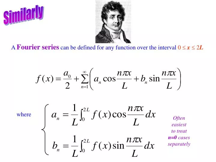
Similarly. A Fourier series can be defined for any function over the interval 0 x 2 L. where. Often easiest to treat n=0 cases separately. Compute the Fourier series of the SQUARE WAVE function f given by. p. 2 p. Note: f(x) is an odd function ( i.e. f(-x) = -f(x) ).

E N D
Similarly A Fourier series can be defined for any function over the interval 0 x 2L where Often easiest to treat n=0 cases separately
Compute the Fourier series of the SQUARE WAVE function f given by p 2p Note:f(x)is an odd function ( i.e.f(-x) = -f(x)) so f(x)cosnxwill be as well, whilef(x)sinnxwill be even.
change of variables: x x'= x- periodicity: cos(X+n) = (-1)ncosX for n = 1, 3, 5,…
for n = 2, 4, 6,… for n = 1, 3, 5,… change of variables: x x'= nx IFf(x) is odd, all an vanish!
change of variables: x xnew= xold- periodicity: sin(X±n) = (-1)nsinX for n = 1, 3, 5,… and vanishing for n = 2, 4, 6,…
for n = 2, 4, 6,… for n = 1, 3, 5,… change of variables: x x'= nx for odd n for n = 1, 3, 5,…
y N = 1 1 N= 5 2 x
Leads you through a qualitative argument in building a square wave http://mathforum.org/key/nucalc/fourier.html Add terms one by one (or as many as you want) to build fourier series approximation to a selection of periodic functions http://www.jhu.edu/~signals/fourier2/ Build Fourier series approximation to assorted periodic functions and listen to an audio playing the wave forms http://www.falstad.com/fourier/ Customize your own sound synthesizer http://www.phy.ntnu.edu.tw/java/sound/sound.html
Fourier transforms of one another
Two waves of slightly different wavelength and frequency produce beats. x 2 1 k k = x NOTE: The spatial distribution depends on the particular frequencies involved
Many waves of slightly different wavelength can produce “wave packets.”
Adding together many frequencies that are bunched closely together …better yet… integrating over a range of frequencies forms a tightly defined, concentrated “wave packet” A staccato blast from a whistle cannot be formed by a single pure frequency but a composite of many frequencies close to the average (note) you recognize You can try building wave packets at http://phys.educ.ksu.edu/vqm/html/wpe.html
The broader the spectrum of frequencies (or wave number) …the shorter the wave packet! The narrower the spectrum of frequencies (or wave number) …the longer the wave packet!
Fourier Transforms Generalization of ordinary “Fourier expansion” or “Fourier series” Note how this pairs “canonically conjugate” variables and t. Whose product must bedimensionless(otherwisee-itmakesno sense!)
Conjugate variables t, time & frequency: What about coordinate position & ???? inverse distance?? rorx wave number, In fact through the deBroglie relation, you can write:
For a well-localized particle (i.e., one with a precisely known position at x = x0) we could write: Dirac -function a near discontinuous spike at x=x0, (essentially zero everywhere except x=x0) with 1 x x x0 x0 such that f(x)≈ f(x0), ≈constant over x-x, x+x
For a well-localized particle (i.e., one with a precisely known position at x = x0) we could write: In Quantum Mechanics we learn that the spatial wave function(x)can be complemented by the momentum spectrum of the state, found through the Fourier transform: Here that’s Notice that the probability of measuring any single momentum value, p, is: What’s THAT mean? The probability is CONSTANT – equal for ALL momenta! All momenta equally likely! The isolated, perfectly localized single packet must be comprised of an infinite range of momenta!
Remember: (k) (x) k0 (x) (k) k0 …and, recall, even the most general whether confined by some potential OR free actually has some spatial spread within some range of boundaries!
Fourier transforms do allow an explicit “closed” analytic form for the Dirac delta function
Let’s assume a wave packet tailored to be something like a Gaussian (or “Normal”) distribution Area within 1 68.26% 1.28 80.00% 1.64 90.00% 1.96 95.00% 2 95.44% 2.58 99.00% 3 99.46% 4 99.99% A single “damped” pulse bounded tightly within a few of its mean postion, μ. +2 -2 -1 +1
For well-behaved (continuous) functions (bounded at infiinity) likef(x)=e-x2/22 Starting from: -i k g'(x) g(x)= e+ikx f(x) we can integrate this “by parts” f(x) is bounded oscillates in the complex plane over-all amplitude is damped at ±
And so, specifically for a normal distribution:f(x)=e-x2/22 differentiating: from the relation just derived: Let’s Fourier transform THIS statement i.e., apply: on both sides! 1 2 ~ ~ ~ F'(k)e-ikxdk 1 2 ~ ei(k-k)xdx ~ (k – k)
1 2 ~ ei(k-k)xdx ~ (k – k) ~ selecting out k=k k k ' ' rewriting as: dk' dk' ' 0 0
Fourier transforms of one another Gaussian distribution about the origin Now, since: we expect: Both are of the form of a Gaussian! x k 1/
x k 1 or giving physical interpretation to the new variable x px h