Download
1 / 97
1.01k likes | 1.17k Views
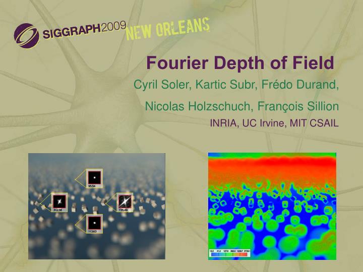
Fourier Depth of Field. Cyril Soler, Kartic Subr, Frédo Durand, Nicolas Holzschuch, François Sillion. INRIA, UC Irvine, MIT CSAIL. Defocus blur is important in photography. Defocus is due to integration over aperture. Lens. Aperture. Image. Pixel p. Defocus. Lens. Aperture. Scene.

E N D
Fourier Depth of Field Cyril Soler, Kartic Subr, Frédo Durand, Nicolas Holzschuch, François Sillion INRIA, UC Irvine, MIT CSAIL
Defocus is due to integration over aperture Lens Aperture Image Pixel p
Defocus Lens Aperture Scene Image Pixel p
Monte Carlo estimate of aperture integral NA primary rays per pixel Aperture Image Integrate at p
Aperture integration is costly NP x NA Primary rays Image Aperture NP pixels NA Aperture samples
Aperture integration is costly Paradox: More blurry image is costlier to compute! 64 x #primary rays of the pinhole image
Observation 1: Image sampling Blurry regions should not require dense sampling of the image
Observation 2: Lens sampling Regions in focus should notrequire profuse sampling of the lens for diffuse objects
Observation 2: Aperture sampling Plane in focus At “sharp” pixels, rays are from same scene point Image Lens Regions in focus should notrequire profuse sampling of the lens for diffuse objects
Observation 2: Aperture sampling Plane in focus Variance depends on reflectance Image Lens Regions in focus should notrequire profuse sampling of the lens for diffuse objects
Goal: Adaptive sampling • Reduce number of primary rays • Adapt image and lens sampling rates based on Fourier bandwidth prediction
Sampling: 1) Image Sample blurry image regions sparsely Reference Our image samples
Sampling: 2) Aperture Sample aperture sparsely for objects in focus 100 4 20
Contributions • Fourier analysis of depth of field for image synthesis • Account for different transport phenomena • Mechanism for propagating local frequency content • Adaptive sampling of image and lens
Related work: Sampling approach • Trace multiple rays per pixel • Correctly account for phenomena • Costly [Cook et al. 87] [Cook et al. 84]
Related work: Image space approach • Post process pinhole image using depth map • Fast although approximate • Correct handling of occlusion is a challenge [Potmesil and Chakravarty 81] [Kraus and Strengert 07] [Kass et al. 06]
Related work: Frequency domain analysis [Ng. 05] [Chai et al. 2000] [Durand et al. 05] [Ramamoorthi and Hanrahan 04]
Typical Algorithm for estimating defocus P= {uniformly distributed image samples} NA // number of aperture samples for each pixel x in P L ← SampleLens(NA) for each sample y in L Sum ← Sum + EstimatedRadiance(x, y) Image (x) = Sum / NA
Our adaptive sampling L ← SampleLens(NA) for each sample y in L Sum ← Sum + EstimatedRadiance(x, y) Image (x) = Sum / NA (P, A) ← BandwidthEstimation() P= {uniformly distributed image samples} NA P= {bandwidth dependent image samples} A = {aperture variance estimate} for each pixel x in P NA proportional to A(x) Reconstruct (Image, P)
Algorithm Bandwidth Estimation Sampling rates over image and lens Estimate radiance rays through image and lens samples Reconstruct image from scattered radiance estimates
Review: Local light field parametrization Angle Space [Durand05]
Review: Local light field as a density 1D Lambertian emitter Local light field Angle Space [Durand05]
Review: Local light field spectrum Power spectrum Local light field Angular frequencies Fourier Transform Spatial frequencies [Durand05]
Review: Transport & Local light field spectra Processes Operations Reflectance Product Transport (free space) Shear (angle) Occlusion Convolution [Durand05]
Our sampled representation Sampled Light field spectrum Light field spectrum Spatial frequencies Angular frequencies • Samples in frequency space • Updated through light transport • Provides • bandwidth (max frequency) • Variance (sum of square frequencies)
Our sampled representation Sampled Light field spectrum Light field spectrum Spatial freq. High spatial frequency High angular frequency Angular freq. • Samples in frequency space • Updated through light transport • Provides • bandwidth (max frequency) • Variance (sum of square frequencies)
Our sampled representation Sampled Light field spectrum Light field spectrum High spatial frequency Low angular frequency Angular freq. • Samples in frequency space • Updated through light transport • Provides • bandwidth (max frequency) • Variance (sum of square frequencies)
Our sampled representation Sampled Light field spectrum Light field spectrum Spatial freq. Max angular freq. Angular freq. • Samples in frequency space • Updated through light transport • Provides • bandwidth (max frequency) • Variance (sum of square frequencies)
Propagating light field spectra Coarse depth image Scene Propagate spectra Aperture Sensor
Propagating light field spectra Coarse depth image Scene Propagate spectra Aperture variance Aperture Image –space bandwidth Sensor
Propagating light field spectra Coarse depth image Scene Propagate spectra Aperture variance Aperture Image –space bandwidth Trace rays Sensor Sparse radiance
Propagating light field spectra Light field incident at P First intersection point P Primary ray through lens center Variance over aperture Aperture Sensor Local image bandwidth
Propagating light field spectra Light field incident at P Reflection First intersection point P Primary ray through lens center Transport through free space Aperture effect Aperture Sensor
Incident light field Angular frequency Spatial frequency • Assume full spectrum • Conservatively expect all frequencies • Simple, no illumination dependence
Reflection: Last bounce to the eye • Convolution by BRDF • Fourier domain: Product of spectra x = Incident light field spectrum BRDF spectrum Light field spectrum after reflection
Reflection: Last bounce to the eye • Convolution by BRDF • Fourier domain: Product of spectra x = Incident light field spectrum BRDF spectrum Light field spectrum after reflection
Transport to aperture • Transport through free space: angular shear of the light field spectrum [Durand05] Angular frequency Spatial frequency
Transport to aperture • Transport through free space • Occlusion: Convolution with blocker spectrum [Durand05] Occluder * = Light field before occlusion Blocker spectrum Light field spectrum after occlusion
Occlusion test • To find occluders for ray through pixel p • Test if depth value at q is in cone of rays Occluder Image p
Occlusion test • To find occluders for ray through pixel p • Test if depth value at q is in cone of rays Occluder Image p q
Occlusion test • To find occluders for ray through pixel p • Test if depth value at q is in cone of rays Occluder Image p q
Operations on sampled spectra f(x) g(x) Draw Samples Y X X+Y
Operations on sampled spectra * f(x) g(x) f(x) g(x) Draw Samples Y X X+Y X+Y Simply add frequency samples and sampled occluder spectra
Transport to aperture • Transport through free space • Occlusion: Convolution with blocker spectrum [Durand05] Occluder * = Light field before occlusion Blocker spectrum Light field spectrum after occlusion
Transport to aperture • Transport through free space • Occlusion • Transport through free space Occluder Angular frequency Spatial frequency