Download
1 / 74
750 likes | 855 Views
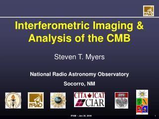
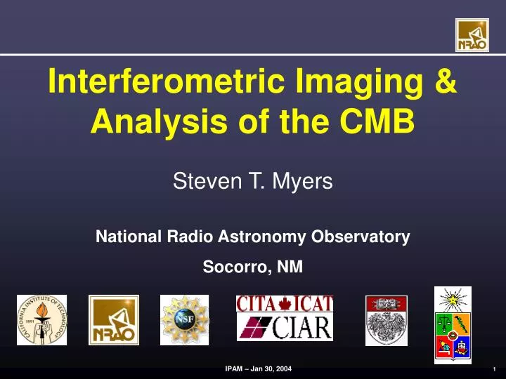
Interferometric Imaging & Analysis of the CMB. Steven T. Myers. National Radio Astronomy Observatory Socorro, NM. Interferometers. Spatial coherence of radiation pattern contains information about source structure Correlations along wavefronts

E N D
Interferometric Imaging & Analysis of the CMB Steven T. Myers National Radio Astronomy Observatory Socorro, NM
Interferometers • Spatial coherence of radiation pattern contains information about source structure • Correlations along wavefronts • Equivalent to masking parts of a telescope aperture • Sparse arrays = unfilled aperture • Resolution at cost of surface brightness sensitivity • Correlate pairs of antennas • “visibility” = correlated fraction of total signal • Fourier transform relationship with sky brightness • Van Cittert – Zernicke theorem
Radio Interferometers • Connected-element “radio” interferometers: • The Very Large Array (VLA) @ New Mexico • Owens Valley Millimeter-wave Array @ California • BIMA Millimeter-wave Array @ California • Coming: • CARMA (combined OVRO & BIMA) • ALMA Millimeter-wave Array @ Chile • CMB interferometers • Ryle Telescope @ UK • DASI @ South Pole • VSA @ Tenerife • CBI @ Chile
Example: The VLA • 27 elements • 25m apertures • Maxiumum baseline 36km (A-config) • Y-pattern, 4 configurations (36km,10km,3.6km,1km)
CMB Interferometers • CMB issues: • Extremely low surface brightness fluctuations < 50 mK • Polarization less than 10% • Large monopole signal 3K, dipole 3 mK • No compact features, approximately Gaussian random field • Foregrounds both galactic & extragalactic • Traditional direct imaging • Differential horns or focal plane arrays • Interferometry • Inherent differencing (fringe pattern), filtered images • Works in spatial Fourier domain • Element gain effect spread in image plane • Limited by need to correlate pairs of elements • Sensitivity requires compact arrays
CMB Interferometers: DASI, VSA • DASI @ South Pole • VSA @ Tenerife
CMB Interferometers: CBI • CBI @ Chile
The Instrument • 13 90-cm Cassegrain antennas • 78 baselines • 6-meter platform • Baselines 1m – 5.51m • 10 1 GHz channels 26-36 GHz • HEMT amplifiers (NRAO) • Cryogenic 6K, Tsys 20 K • Single polarization (R or L) • Polarizers from U. Chicago • Analog correlators • 780 complex correlators • Field-of-view 44 arcmin • Image noise 4 mJy/bm 900s • Resolution 4.5 – 10 arcmin
CBI Instrumentation • Correlator • Multipliers 1 GHz bandwidth • 10 channels to cover total band 26-36 GHz (after filters and downconversion) • 78 baselines (13 antennas x 12/2) • Real and Imaginary (with phase shift) correlations • 1560 total multipliers
CBI Operations • Observing in Chile since Nov 1999 • NSF proposal 1994, funding in 1995 • Assembled and tested at Caltech in 1998 • Shipped to Chile in August 1999 • Continued NSF funding in 2002, to end of 2004 • Chile Operations 2004-2005 pending proposal • Telescope at high site in Andes • 16000 ft (~5000 m) • Located on Science Preserve, co-located with ALMA • Now also ATSE (Japan) and APEX (Germany), others • Controlled on-site, oxygenated quarters in containers • Data reduction and archiving at “low” site • San Pedro de Atacama • 1 ½ hour driving time to site
The Cosmic Microwave Background • Discovered 1965 (Penzias & Wilson) • 2.7 K blackbody • Isotropic • Relic of hot “big bang” • 3 mK dipole (Doppler) • COBE 1992 • Blackbody 2.725 K • Anisotropies 10-5
Thermal History of the Universe Courtesy Wayne Hu – http://background.uchicago.edu
CMB Anisotropies • Primary Anisotropies • Imprinted on photosphere of “last scattering” • “recombination” of hydrogen z~1100 • Primordial (power-law?) spectrum of potential fluctuations • Collapse of dark matter potential wells inside horizon • Photons coupled to baryons >> acoustic oscillations! • Electron scattering density & velocity • Velocity produces quadrupole >> polarization! • Transfer function maps P(k) >> Cl • Depends on cosmological parameters >> predictive! • Gaussian fluctuations + isotropy • Angular power spectrum contains all information • Secondary Anisotropies • Due to processes after recombination
Primary Anisotropies Courtesy Wayne Hu – http://background.uchicago.edu
Primary Anisotropies Courtesy Wayne Hu – http://background.uchicago.edu
Secondary Anisotropies Courtesy Wayne Hu – http://background.uchicago.edu
Images of the CMB WMAP Satellite BOOMERANG ACBAR
WMAP Power Spectrum Courtesy WMAP – http://map.gsfc.nasa.gov
CMB Polarization • Due to quadrupolar intensity field at scattering • E & B modes • E (gradient) from scalar density fluctuations predominant! • B (curl) from gravity wave tensor modes, or secondaries • Detected by DASI and WMAP • EE and TE seen so far, BB null • Next generation experiments needed for B modes • Science driver for Beyond Einstein mission • Lensing at sub-degree scales likely to detect • Tensor modes hard unless T/S~0.1 (high!) Hu & Dodelson ARAA 2002
The Fourier Relationship • The aperture (antenna) size smears out the coherence function response • Like a double-slit experiment with widening slits • Interference plus diffraction pattern • Lose ability to localize wavefront direction = field-of-view • Small apertures = wide field • An interferometer “visibility” in the sky and Fourier planes:
The uv plane and l space • The sky can be uniquely described by spherical harmonics • CMB power spectra are described by multipole l ( the angular scale in the spherical harmonic transform) • For small (sub-radian) scales the spherical harmonics can be approximated by Fourier modes • The conjugate variables are (u,v) as in radio interferometry • The uv radius is given by l / 2p • The projected length of the interferometer baseline gives the angular scale • Multipole l = 2pB / l • An interferometer naturally measures the transform of the sky intensity in l space
CBI Beam and uv coverage • 78 baselines and 10 frequency channels = 780 instantaneous visibilities • Frequency channels give radial spread in uv plane • Pointing platform rotatable to fill in uv coverage • Parallactic angle rotation gives azimuthal spread • Beam nearly circularly symmetric • Baselines locked to platform in pointing direction • Baselines always perpendicular to source direction • Delay lines not needed • Very low fringe rates (susceptible to cross-talk and ground)
CMB peaks smaller than this ! Field of View and Resolution • An interferometer “visibility” in the sky and Fourier planes: • The primary beam and aperture are related by: CBI:
Power Spectrum and Likelihood • Statistics of CMB (Gaussian) described by power spectrum: Construct covariance matrices and perform maximum Likelihood calculation: Break into bandpowers
Power Spectrum Estimation • Method described in Paper IV (Myers et al. 2003) • Large datasets • > 105 visibilities in 6 x 7 field mosaic • ~ 103 independent • Gridded “estimators” in uv plane • Convolution with aperture matched filter • Fast! Reduces number of points for likelihood • Not lossless, but information loss insignificant • Construct covariance matrices for gridded points • Maximum likelihood using BJK method • Output bandpowers • Wiener filtered images constructed from estimators
Covariance of Visibilities • Write with operators • Covariance • Problem • Size of v, P >105 visibilities, 104 distinct per mosaic pointing! v = P t + e < v v†> = P < t t † > P† + <ee†>
Gridded Visibilities • Convolve with “matched filter” kernel • Kernel • Normalization • Returns true t for infinite continuous mosaic D = Q v + Q v* Deal with conjugate visibilities
Covariance of Gridded Visibilities < DD†> = Q < v v † > Q† + conjg. =Q P < t t † > P † Q† + Q <ee†> Q† + conjg. • Covariance • Or • Problem • Reduced to 103 to 104 grid cells • Complicates covariance calculation, loss of information D = R t + n R = Q P + Q P n = Q e < DD†> = R < t t † > R† + <nn†>
Tests with mock data • The CBI pipeline has been extensively tested using mock data • Use real data files for template • Replace visibilties with simulated signal and noise • Run end-to-end through pipeline • Run many trials to build up statistics
Wiener filtered images • Covariance matrices can be applied as Wiener filter to gridded estimators • Estimators can be Fourier transformed back into filtered images • Filters CX can be tailored to pick out specific components • e.g. point sources, CMB, SZE • Just need to know the shape of the power spectrum
Example – Mock deep field Noise removed Raw CMB Sources
CBI 2000 Results • Observations • 3 Deep Fields (8h, 14h, 20h) • 3 Mosaics (14h, 20h, 02h) • Fields on celestial equator (Dec center –2d30’) • Published in series of 5 papers (ApJ July 2003) • Mason et al. (deep fields) • Pearson et al. (mosaics) • Myers et al. (power spectrum method) • Sievers et al. (cosmological parameters) • Bond et al. (high-l anomaly and SZ) pending
Calibration and Foreground Removal • Calibration scale ~5% • Jupiter from OVRO 1.5m (Mason et al. 1999) • Agrees with BIMA (Welch) and WMAP • Ground emission removal • Strong on short baselines, depends on orientation • Differencing between lead/trail field pairs (8m in RA=2deg) • Use scanning for 2002-2003 polarization observations • Foreground radio sources • Predominant on long baselines • Located in NVSS at 1.4 GHz, VLA 8.4 GHz • Measured at 30 GHz with OVRO 40m • Projected out in power spectrum analysis
CBI Deep Fields 2000 • Deep Field Observations: • 3 fields totaling 4 deg^2 • Fields at d~0 a=8h, 14h, 20h • ~115 nights of observing • Data redundancy strong tests for systematics
CBI 2000 Mosaic Power Spectrum • Mosaic Field Observations • 3 fields totaling 40 deg^2 • Fields at d~0 a=2h, 14h, 20h • ~125 nights of observing • ~ 600,000 uv points covariance matrix 5000 x 5000
Cosmological Parameters wk-h: 0.45 < h < 0.9, t > 10 Gyr HST-h: h = 0.71 ± 0.076 LSS: constraints on s8 and G from 2dF, SDSS, etc. SN: constraints from Type 1a SNae
SZE Angular Power Spectrum [Bond et al. 2002] • Smooth Particle Hydrodynamics (5123) [Wadsley et al. 2002] • Moving Mesh Hydrodynamics (5123) [Pen 1998] • 143 Mpc 8=1.0 • 200 Mpc 8=1.0 • 200 Mpc 8=0.9 • 400 Mpc 8=0.9 Dawson et al. 2002
Constraints on SZ “density” • Combine CBI & BIMA (Dawson et al.) 30 GHz with ACBAR 150 GHz (Goldstein et al.) • Non-Gaussian scatter for SZE • increased sample variance (factor ~3)) • Uncertainty in primary spectrum • due to various parameters, marginalize • Explained in Goldstein et al. (astro-ph/0212517) • Use updated BIMA (Carlo Contaldi) Courtesy Carlo Contaldi (CITA)
LSS parameters from Surveys Priors Flat HST-h Courtesy J.R. Bond
New : Calibration from WMAP Jupiter • Old uncertainty: 5% • 2.7% high vs. WMAP Jupiter • New uncertainty: 1.3% • Ultimate goal: 0.5%