Download
1 / 26
260 likes | 357 Views
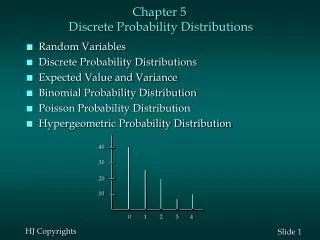
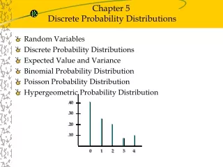
Chapter 5 Discrete Probability Distributions. Probability Experiment. A probability experiment is any activity that produces uncertain or “random” outcomes. Random Variable. A random variable is a rule or function that translates the outcomes of a probability experiment into numbers.

E N D
Probability Experiment A probability experiment is any activity that produces uncertain or “random” outcomes
Random Variable A random variable is a rule or function that translates the outcomes of a probability experiment into numbers.
Table 5.1 Illustrations of Random Variables
Discrete Random Variable A discrete random variable has separate and distinct values, with no values possible in between.
Continuous Random Variable A continuous random variable can take on any value over a given range or interval.
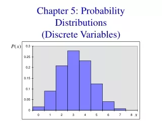
Probability Distribution A probability distribution identifies the probabilities that are assigned to all possible values of a random variable.
Producing a Discrete Probability Distribution Step 1: Defining the Random Variable Step 2: Identifying Values for the Random Variable Step 3: Assigning Probabilities to Values of the Random Variable
Figure 5.1 Probability Tree for the Management Training Example Outcomex P(x) J (.7) (1) S∩J 2 .63 Jones Passes S (.9) Smith Passes J' (.3) (2) S∩J’ 1 .27 Jones Fails J (.7) (3) S'∩J 1 .07 Jones Passes S' (.1) Smith Fails J' (.3) (4) S'∩J’ 0 .03 Jones Fails
Probability Distribution for the Training Course Illustration
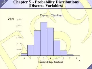
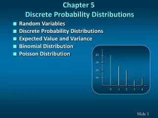
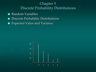
0 1 2 x Figure 5.2 Graphing the Management Training Distribution P(x) .6 .3 .1 Number of Managers Passing
Expected Value for a (5.1) Discrete Probability Distribution E(x) = xP(x)
H (.4) 3 Heads .064 H (.4) T (.6) 2 Heads .096 H (.4) H (.4) .096 2 Heads T (.6) T (.6) 1 Head .144 H (.4) .096 2 Heads H (.4) T (.6) 1 Head .144 T (.6) H (.4) 1 Head .144 T (.6) T (.6) 0 Heads .216 Figure 5.3 Probability Tree for the Coin Toss Example
The Binomial Conditions • The experiment involves a number of “trials”— that is, repetitions of the same act. We’ll use n to designate the number of trials. (2) Only two outcomes are possible on each of the trials. This is the “bi” part of “binomial.” We’ll typically label one of the outcomes a success, the other a failure. (3) The trials are statistically independent. Whatever happens on one trial won’t influence what happens on the next. (4) The probability of success on any one trial remains constant throughout the experiment. For example, if the coin in a coin-toss experiment has a 40% chance of turning up heads on the first toss, then that 40% probability must hold for every subsequent toss. The coin can’t change character during the experiment. We’ll normally use p to represent this probability of success.
Expected Value for a (5.5) Binomial Distribution E(x) = nּ p
Variance for a Binomial Distribution (5.6) s2 = nּpּ(1-p)
Standard Deviation for a (5.7) Binomial Distribution s =
P(x) Positively Skewed 0 1 2 3 4 5 6 x P(x) 0 1 2 3 4 5 6 x P(x) Negatively Skewed 0 1 2 3 4 5 6 x Figure 5.4 Some Possible Shapes for a Binomial Distribution Symmetric
The Poisson Conditions • We need to be assessing probability for the number of occurrences of some event per unit time, space, or distance. (2) The average number of occurrences per unit of time, space, or distance is constant and proportionate to the size of the unit of time, space or distance involved. (3) Individual occurrences of the event are random and statistically independent.
P(x) .3 .2 .1 0 1 2 3 4 5 6 x mean = l=1 Figure 5.5 Graphing the Poisson Distribution for l = 1
P(x) .3 .2 .1 Figure 5.6 Matching Binomial and Poisson Distributions P(x) .3 .2 .1 BINOMIAL n= 20, p = .10 0 1 2 3 4 5 6 x POISSON l = 2 0 1 2 3 4 5 6 x