Download
1 / 8
80 likes | 187 Views
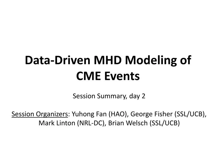
Data-Driven MHD Modeling of CME Events. Session Summary, day 2 Session Organizers : Yuhong Fan (HAO), George Fisher (SSL/UCB), Mark Linton (NRL-DC), Brian Welsch (SSL/UCB). Slava Titov : "Structural Analysis of the Coronal Mag- netic Field: How Can It Be Used in Models of CMEs?" .

E N D
Data-Driven MHD Modeling of CME Events Session Summary, day 2 Session Organizers: Yuhong Fan (HAO), George Fisher (SSL/UCB), Mark Linton (NRL-DC), Brian Welsch (SSL/UCB)
SlavaTitov: "Structural Analysis of the Coronal Mag-netic Field: How Can It Be Used in Models of CMEs?" Start: review of separatrix surfaces, and quasi-separatrix layers (QSLs) as sites of reconnection; Q := "squashing factor" quantifies rate of change of field-line connectivity near a QSL Q enables: • localising preferred sites of reconnection, i.e., quasi-separators • identifying building blocks, e.g., erupting and non- strands of flux ropes (3) determine evolving fluxes for each blocks (4) relate observable structures to building blocks: • H-alpha flare ribbons, • EUV dimmings, • X-ray sigmoids
Relation to observational features t=32 (≈ 38 min after the CME onset)
Roussev:Use Dynamic Flux Emergence Simulations (w/Galsgaard& Archontis) to Drive Coronal Model • This enables driving with more self-consistent boundary conditions. - required rescaling β from photospheric to coronal values, and decreasing peak field strength. • Flux rope forms, and erupts; post-eruption field consists of two flux ropes, which form a “double J” structure • synthetic X-ray emission resembles observed sigmoids • Topology matters: nulls & QSLs play important roles (cf., Titov) • Footpoints of erupting rope do not remain stationary, but move across surface as eruption proceeds. • Flux rope does not remain intact: after eruption, two flux ropes are formed, linking “core" of emerged field to external field
Magnetic Field Geometry at Later Times t = 68 min t = 3 h
Several “data inspired” simulations of actual eruptions were presented: Zuccarello; Fan; Jin. Models had varying degrees of thermodynamic realism. Fan’s CME was slower than the observed CME: • Fan: Rescaling must preserve height profile of B. • Fisher: If you get a 1000 km/sec eruption, how do you change parameters to achieve a 2000 km/sec eruption? • Mikic: To increase eruption energy, confine the pre-eruption field more strongly. • Fisher: So, for instance, if you want to build a pipe bomb, you should not use a cardboard tube, you should instead use a metal tube. • Mikic: Yes, you want to prevent expansion for a while… Meng Jin studied a CME shock with one-T and two-T models: • 1T: 9 MK precursor far ahead of shock • 2T: 3 MK peak e- T, 100 MK peak proton T (Mach #’s near 4) • Heat flux saturation (not in model) was discussed
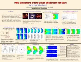
Reinard: Charge-state predictions from MHD CME simulations can be used to interpret in situ observations. QFe derived from Breakout model QFe derived from Flux cancellation QFeobservations for the two May 19-21, 2007 MCs MC1 STA MC2 ACE STB

![Data Modeling [Comparison of data modeling techniques ]](https://cdn0.slideserve.com/205866/data-modeling-comparison-of-data-modeling-techniques-dt.jpg)
![MHD Modeling [Riley et al.]](https://cdn1.slideserve.com/3310320/slide1-dt.jpg)

![Data Modeling [Comparison of data modeling techniques ]](https://cdn3.slideserve.com/6795343/data-modeling-comparison-of-data-modeling-techniques-dt.jpg)