Download
1 / 53
540 likes | 649 Views
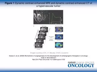
Analysis of Contrast-Enhanced Dynamic MR Lung Images. Geir Torheim 1,2 , Giovanni Sebastiani 3 , Tore Amundsen 2 , Fred Godtliebsen 4 , Olav Haraldseth 1,2.

E N D
Analysis of Contrast-Enhanced Dynamic MR Lung Images Geir Torheim1,2, Giovanni Sebastiani3, Tore Amundsen2, Fred Godtliebsen4, Olav Haraldseth1,2 1MR Center Medical Section, Norway, 2Norwegian University of Science and Technology, Trondheim, Norway, 3Istituto per le Applicazioni del Calcolo, C.N.R., Rome, Italy, 4Université de Mons-Hainaut, Mons, Belgium, and University of Tromsø, Tromsø, Norway
Structure of the talk • Introduction • What is magnetic resonance imaging (MRI)? • What is dynamic MRI ? • Pulmonary embolism • Dynamic Lung MRI • Part I Motion correction • Part II Noise reduction using Bayes • Part III Noise reduction using novel filter
What is Magnetic Resonance Imaging? • The patient is placed in a magnet • A radio signal is sent into the body • The signal causes the body to generate a radio signal • The radio signal from the body is received by antennas • A computer turns the data into an image
What is Dynamic MR Imaging? • A series of images is acquired over time • The images cover the same anatomical area • The series monitors changes with time • Contrast agent administration • Functional imaging of the brain
Intensity Time Parametric Image
Pulmonary Embolism Cause: Deep Vein Thrombosis Incidence: 0.25 % in the Western countries Mortality: 30 % of non treated (hosp.) < 5 % of treated Treatment: Bleeding occurrence: 0.5-1 % (fatal) 10-30 % (non-fatal)
Pulmonary Embolism Large vessels:Capillary phase: • Pulmonary angiography • Perfusion scintigraphy • MR angiography • MR Perfusion Imaging
PE: A problematic diagnosis Present imaging techniques: • X-Ray pulmonary angiography • perfusion and ventilation radionuclide scanning (scintigraphy) • spiral CT • X-Ray peripheral venography (DVT) • Have side effects • Need for more accurate diagnosis
Dynamic Lung MRI • Gives perfusion information with higher spatial resolution than scintigraphy • No irradiation • Can be combined with other MRI techniques • MRA of lung • MRA of lower extremities • MRA: Magnetic Resonance Angiography
Problems in dynamic lung MRI • Non-rigid deformation of the lungs • Long acquisition times prohibits breath hold • Low Signal-to-Noise-Ratio (SNR) • Due to low tissue content in the lungs Can post processing solve both problems ?
Part I Motion Correction
Motion correction • The lung was modeled as a pump, the diaphragm being the “piston” • An automatic method for detection of diaphragm was constructed
Motion correctionStrategy • Detect diaphragm in every frame • Detect the rest of the lung shape • Combine 1 and 2 into lung masks 1 2 3
Motion correction • The diaphragm has a parabolic shape • The following equations were formulated: y = a1(x - xm)2 + ym if x <= xm y = a2(x - xm)2 + ym if x > xm • These equations describe two parabolas interconnected in the point (xm, ym)
Motion correction • The parameters to be found are: a1, a2, xm and ym • The parameters were related to pixel intensities by means of the signed X gradient along the parametric curve
Motion correction • To find the optimal parameters, simulated annealing was used • The Metropolis algorithm was implemented • The method always accepts moves when the energy goes down, and sometimes accepts moves when the energy goes up
- - = ( ) /( ) E E sT p e 2 1 Motion correctionSimulated annealing • p is the probability of stepping to the new energy state • E2 is the energy of the proposed state • E1 is the current energy state • T is temperature • s is a scaling factor to compensate for differences in intensity levels from one frame to the next
Motion correctionSimulated annealing • At each step, the best parameters were saved • The globally best parameters were used • The energies were collected in an array • When the standard deviation of the energies were below a threshold, the algorithm halted • The temperature was decreased when the energy decreased
Motion correction • To increase the speed and accuracy: • A bounding box was drawn around the area of the diaphragm • This area was visualized by calculating the difference between the maximum and minimum intensity projections
Motion correction Bounding boxes drawn on the difference image
Motion correction Automatic detection of diaphragm Pre contrast Peak Post contrast
Motion correction • To get a good delineation of the upper parts of the lungs, a maximum intensity projection of all the frames was created • A spline-based ROI was drawn manually on the maximum intensity projection image
Motion correction Manually drawn masks on a maximum intensity projection image
- m u = - - u n n a m ( l a ) u n n , , m n n n l n - l u n n m n a m,n l n a l,n Motion correctionMapping of pixels Reference lung Lung to be aligned
Motion CorrectionExamples Time Intensity Curves After motion correction Before motion correction
Part II Noise reduction Bayesian approach
Bayesian approach to Noise Reduction • The measured image y is expressed as y = x + e • x is the true, noise free image • y is the observed image • e is Gaussian random noise
µ p ( x | y ) p ( y | x ) p ( x ) Bayesian approach to Noise Reduction • Bayes Theorem • Models for p(x) and p(y|x) were formulated. • These models require two (three) parameters to work
Bayesian approach to Noise Reduction • Assuming independent, Gaussian noise p(y|x) becomes 2 - = ps - - s 2 / 2 2 n p ( y | x ) ( 2 ) exp[ y x / 2 ] n is the number of pixels in the image. 2 is the noise variance, estimated from a Region Of Interest (ROI) positioned in the liver.
é ù å = - p ( x ) ( 1 / Z ) exp V ( x ) ê ú C ë û Î y C Bayesian approach to Noise Reduction Assuming x can be modeled as a Markov Random field, p(x) is given by Gibbs distribution: where Z is a constant and Vc is the potential
[ ] x = - b x V ( ) ln p ( ) Bayesian approach to Noise Reduction V was modeled as follows: is a smoothing parameter
é ù å å + = ( 1 ) ( ) ( 0 ) ( ) k k k p p w p / w p , ê ú i i ij j jt t ë û j t Bayesian approach to Noise Reduction p was discretized and estimated as follows: • wij is the value of the Gaussian density N(0,2s2) corresponding to i-j • pj(0) is the empirical distribution of the neighbor differences of y
Bayesian approach to Noise Reduction • The contrast agent is changing the contrast behavior • Therefore, two smoothing parameters were estimated • The “best” parameters values were found by smoothing two images iteratively using different values • The “best” value was the one which minimized the difference between histograms from an average image and the denoised image
Bayesian approach to Noise ReductionEffect of smoothing parameter Original image = 0.15 = 0.3 = 0.5
Bayesian approach to Noise ReductionExamples Time Intensity Curves Time intensity curve before denoising Time intensity curve after denoising
Bayesian approach to Noise ReductionResults Parametric images of a patient with Pulmonary Embolism Original data After motion correction After motion correction+Bayes
Part III Noise reduction An alternative approach
= r + e Z ( x , y , t ) , ijk i j k ijk A novel time series filter1 Assuming gaussian additive noise: • Z: The observed image • : The true image • : Independent identically distributed Gaussian noise 1Described in a paper submitted to IEEE Transactions on Medical Imaging
= ( x , y , t ) B A , r ˆ p q r pqr pqr n n m å å å - - = 1 2 B m n K K K L Z , pqr hpi hqj hrk gpqij ijk = = = i 1 j 1 k 1 n n m å å å - - = 1 2 A m n K K K L . pqr hpi hqj hrk gpqij = = = i 1 j 1 k 1 A novel time series filter
( ) = - L L Z Z pq ij gpqij g m å - = 1 Z m Z . ij ijk = k 1 A novel time series filter Khpi = Kh(xp-xi), Khqj = Kh(yq-yj), Khrk = Kh(tr-tk) Kh( ) = h-1K( /h), Lg( ) = g-1L( /g) L and K are Gaussian kernels
A novel time series filter • The filter can be viewed as an extension of the Nadaraya-Watson estimator • The extention basically consists of the L term • The purpose of the L term is to use only similar curves in the smoothing process
A novel time series filter Three parameters need to be specified: • hxy - Controls the degree of smoothing in x-y plane • ht - Controls the degree of smoothing along time • g - Controls how similar curves must be in order to be included in the smoothing
s 2 2 = g m A novel time series filterParameter settings g was set using the following rule: m is the number of frames and is the noise standard deviation
1 = h ( t ) 2 ¢ ¢ r 2 1 / 5 (( ) ) A novel time series filterParameter settings ht was set to a variable bandwidth function h(t) which was found by the following formula: hxy was found by trial and error
After motion correction+novel filter After motion correction+Bayes Novel filter vs. Bayesian approach Parametric images of a patient with Lung Embolism After motion correction
Summary Part I • A model based method for aligning lung images was implemented • The method performs well on noisy data with little contrast • A mask had to be drawn manually on each slice, however, all processing on individual frames was automatic
Summary part II • A Bayesian noise reduction method was implemented • The method reduces noise without losing much edge information • The method is completely automatic apart from a simple ROI drawing • A drawback is the long processing time