Download
1 / 34
340 likes | 595 Views
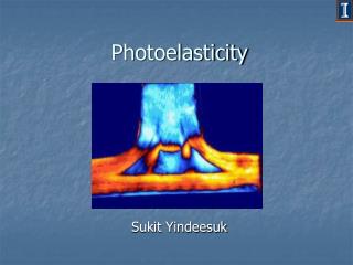
Obstacles Encountered in Calculating the Stress Tensor Using Thermoelasticity and Photoelasticity. Deonna Woolard Department of Physics Randolph-Macon College Ashland, Virginia CS-AAPT Fall 2000 Meeting. History of Photoelasticity.

E N D
Obstacles Encountered in Calculating the Stress Tensor Using Thermoelasticity and Photoelasticity Deonna Woolard Department of Physics Randolph-Macon College Ashland, Virginia CS-AAPT Fall 2000 Meeting
History of Photoelasticity • 1811 David Brewster (calves’ feet jelly birefringent under pressure) • 1853 James Maxwell (one-dimensional photoelastic theory) • 1900 Coker Polariscope (designed the standard polariscope) • 1979 Muller and Saackel (photoelasticity + image processing) • 1980’s Digital image processing on photoelastic fringes • 2000 New polariscopes cheaper cameras, better image quality, algorithms for automation
Photoelasticity E Elastic Modulus Poisson’s Ratio Nn Normal Incidence Fringe Order Wavelength k Strain-optic Coefficient t Thickness of coating Polarizer 1/4 Wave Plate Light Source Photoelastic Coating Test Part 1/4 Wave Plate Polarizer observer
Photoelastic Fringes Isoclinic Fringes (Plane Polarization) Isochromatic Fringes (Circular Polarization)
History of Thermoelasticity • 1805 John Gough (rubber changed temperature when stretched) • 1851 Lord Kelvin (thermoelastic theory) • 1967 Milo Belgen (first TE lab instrument - NASA Langley) • 1974 SPATE (first commercial instrument -- point sensor) • 1990 Thermoelasticity with commercial radiometer (Full-field image by rastering: Cramer and Welch -- NASA Langley) • 2000 New Bolometers (full-field with a higher density of pixels at a lower cost)
Thermoelasticity Coefficient of Thermal Expansion Absolute Temperature Density Cp Specific Heat x, y Principal Stresses
Thermoelastic Images Central hole in a plate under uniaxial tension. The asymmetry is a result of a fatigue crack. Aircraft door latch fitting. Hot spots identify stress concentrations.
Thermoelastic Images For T = 1 mK Material Stress Steel 150 psi (1.0 MPa) Aluminum 60 psi (0.4 Mpa) Epoxy 8 psi (0.06 Mpa) To improve measurements, temperature changes are repeated and time-averaged with a continuous dynamic loading.
Combining Thermoelastic and Photoelastic Data Thermoelasticity + Photoelasticity = Full Stress Tensor Field
Comparison Photoelasticity Thermoelasticity • Full-field, non contact • High emissive surface(flat black paint) • Photon starved • Sum of the principal stresses • Full-field, non contact • Birefringent Coating and Reflective backing(polycarbonates, epoxies) • Photon abundant • Difference of the principal stresses plus the principal stress direction
Surface Coating Characteristics Birefringent Coating Reflective Backing test object Opaque in the 3-5 µm IR band > 500 µm
Photoelastic/Thermoelastic Data Thermoelastic Response Photoelastic Response Hole in a Plexiglas plate under uni-axial tension
Load Setting and a Strain Witness Coating • TE is a quasi-static stress measurement while PE is a static stress measurement PE measurement at the mean load setting in TE Cramer, Dawicke, and Welch (1992) and Barone and Patterson (1996) • PE coatings are plastic based and act as an insulatorattenuating the thermoelastic response Very thick coatings and high frequencies Signal generated by the coating rather than the substrate MacKenzie (1989), Welch and Zickel (1993), Barone and Patterson (1998)
Data Images of Varying Pixel Sizes Thermoelastic Image (DT1000) 127 x 128 Photoelastic Image (Digital Camera) 110 x 235
Thermoelastic Errors • Incorrect calibration • Movement of the edge due to cyclic loading • Detector averages data from the specimen and the adjacent free space • Can be minimized but not eliminated
Sources of Photoelastic Error • Optical elements and test object not perpendicular to the light path • Quarter-wave plate mismatch • Non-retroreflective backing • Material inhomogeneities • Spatial and temporal variations of light
Photoelastic Model • Applied stress causes clear material to become optically anisotropic • Two light waves traveling in medium: ordinary and extraordinary waves • Interference between the two waves causes fringe patterns • Linear light yields isoclinic fringes (direction of principal stresses) • Circular light yields isochromatic fringes (difference of principal stresses) • Complicated to model wave propagation in anisotropic media
Photoelastic Model Polarizer and analyzer shown crossed which results in “dark field” if no birefringence in coating y y’ x’ • Lab frame is (x,y) • Rotated coordinate system (x’,y’) is the local “optical axis” x z polarizer analyzer Electromagnetic boundary value problem solved in coordinates aligned with principal optic axes
Electromagnetic Wave Theory Stress/Strain slight density change modification of n Stress (optically isotropic) (optically uniaxial) Impermittivity Tensor Principal index of refraction
Electromagnetic Wave Theory (stress) (strain) (Elastic stiffness constants) ordinary wave extraordinary wave Phase Velocity
Anisotropic Electromagnetic Boundary Value Problem I M R d
Finite Element Analysis x xy y
Experimental versus Theory 0º Isoclinic Fringe Pattern for a PMMA with a central hole under uni-axial tension.
Depolarization and Oblique Incidence Effects on 0º Isoclinics
Combining Thermoelastic and Photoelastic Data at the Pixel Level
Stress Resolution: Uncertainty in Principal Angle x(psi) y (psi)xy (psi) ° 943 -120.9 0 0.5° 942.92 -120.82 9.28 1° 942.68 -120.58 18.56 2° 942.70 -119.60 37.11 3° 940.09 -117.99 55.60 4° 937.82 -115.72 74.03 error 0.5% 4.3% Large
Stress Resolution: Uncertainty in x -y x -y x(psi) y (psi)xy (psi) 1063.9 943-120.9 0 -5% 916.40 -94.3 0 -10% 889.81 -67.70 0 -20% 836.61 -14.51 0 +5% 969.60 -147.50 0 +10% 996.20 -174.10 0 +20% 1049.39 -227.29 0
Stress Resolution: Combined Photoelastic Errors x -y x(psi) y (psi)xy (psi) 0° 1063.9 943-120.9 0 2° +5% 968.24 -146.14 38.96 2° +10% 944.77 -172.67 40.81 2° -5% 915.17 -93.07 35.25 2° -10% 888.64 -66.54 33.39 errors: 3-6% 21-45% Large
Summary • Thermoelastic + Photoelastic Stress Analysis provides the full field stress tensor • Stress systems linked through a common coating • Theoretical isoclinics are consistent with laboratory observations • Depolarization causes movement of the isoclinic lines and degradation of the isochromatic fringes • Depolarization effects the accurate determination of the full-field stress tensor components
Future • Continue to look at the depolarization effect on the isoclinic fringes • Photo/thermoelastic camera being developed at the University of Sheffield, UK • My continued contribution to the field????? • Find the balance between research, teaching, and committee meetings!