Download

1 / 79
800 likes | 1.03k Views
7.Effective medium. Upscaling problem Backus averaging O’Doherty-Anstey approximation Reuss and Voigt models Bio-Gassmann model Hertz-Mindlin model. Upscaling problem. Does seismic wave see the thin-layering?. Upscaling problem. From microscopic to macroscopic scale

E N D
7.Effective medium • Upscaling problem • Backus averaging • O’Doherty-Anstey approximation • Reuss and Voigt models • Bio-Gassmann model • Hertz-Mindlin model
Upscaling problem Does seismic wave see the thin-layering?
Upscaling problem • From microscopic to macroscopic scale • From pore (graine) scale (millimeters) • From log-scale (centimeteers)
Upscaling problem • Traditionally, upscaling has meant upscaling of reservoir petrophysical properties and flow parameters dedicated for reservoir fluid flow simulation. However, due to the progresses mentioned above, there is a need to extend the concept of upscaling of geological models, for rock physics properties, seismic modelling and analysis. For instance, in 4D history matching, the need for up and downscaling might differ from the traditional concept of upscaling.
Backus averaging • Sequential Backus Averaging is a method of averaging the properties of a stack of thin layers so they are similar to average properties of a single thick layer. Figure 7.1. The Backus averaging scheme
Backus averaging • The advantage of Sequential Backus Averaging is that no artificial "blocks" are introduced into the geology during the upscaling of the well-log data. In this example the density log is blocky, but the compressional- and shear-wave velocity logs have gradational tops and appear thicker. Blocking would distort the amplitudes. Furthermore, if blocking were based solely upon either the density or the sonic curves, the result would be wrong for the other curve. Figure 7.2. The Backus averaging versus blocking averaging
Backus averaging • Thin beds appear thinner at oblique incidence angles. Figure 7.3. The thin beds
Backus averaging • At nonnormal incidence, the averaging operator must be adjusted to include the apparent bed thinning. Figure 7.4. Adjusting of averaging operator
Backus averaging • The offset synthetic shows differing AVO signatures for the same elastic property contrasts, associated with step-functions, blocky beds, and gradational interfaces. Figure 7.5. AVO signatures from different models
Backus averaging (7.1)
Backus averaging (7.2) (7.3) How many combinations of the stiffness coefficients enter these matrices?
Backus averaging (7.4) (7.5)
The effective vertical velocity from Backus averaging (7.6) Stovas and Arntsen, 2003
Layering Figure 7.6. The layering effect (each model computed by compression and doubling of the previous one)
Reflection-transmission versus layering and contrast Figure 7.7. The reflection (bottom)and transmission (top) responses with different contrasts (to the right is 4 times larger).
Binary medium (multiples) Figure 7.8. Multiples contribution into the reflection response
Propagation versus contrast Figure 7.9. Transmission from thin layer model (change in r due to change in r only)
Effective properties versus net-to-gross Figure 7.10. Effective properties from Backus averaging in a binary medium Stovas, Landro and Avseth, 2004
Turbidite sequence from Ainsa basin Figure 7.11. Turbidite system as an example of binary medium
Binary medium (7.7) (7.8) (7.9)
Binary medium (7.10) (7.11) The propagator matrix is not unitary (7.12)
Binary medium From the characteristic equation (7.13) we compute the eigenvalues (7.14)
Binary medium The propagating regime with complex eigenvalues and the blocking regime with real eigenvalues: (7.15)
Propagating and blocking regimes Figure 7.12. Re a as a function of frequency versus layering and contrast. Filled low frequency area relates to an effective medium, next coming gap relates to transition medium. The interchanging of these zones is repeatable.
Velocity limits The time average limit means that the pulse width is much less than the propagation time through the cycle) (7.16) The effective medium limit can be computed assuming phases being small (low frequency limit) (7.17) (7.18) The geometrical average limit
Velocity limits versus volume fraction Figure 7.13. Velocity versus fraction. The larger reflection coefficient the more deviation between time-average and effective medium velocities. The position for maximum difference between them moving to high values of volume fraction with r increase.
Stack of binary layers The propagator matrix can be represented by the eigenvalue decomposition (7.19) (7.20) (7.21)
Stack of binary layers Product of M cycles (7.22) Transmission and reflection response (7.23)
Stack of binary layers Propagating regime Blocking regime (7.24) (7.25) (7.26)
Stack of binary layers Propagating regime (7.27) (7.28)
Stack of binary layers Blocking regime (7.29) (7.30)
Stack of binary layers Figure 7.14. cos a as a function of frequency versus layering and contrast (blue line is for the reference time average medium). Stovas and Ursin, 2005
Stack of binary layers Figure 7.15. Amplitude C as a function of frequency versus layering and contrast (the gaps relates to the extremely large values).
Stack of binary layers Figure 7.16. Transmission response versus layering and contrast. Note the difference between TRT (transmission time for time average medium) and TEM (transmission time for effective medium). Weak transmission for r=0.87 and Model M16 is due to the wavelet spectrum is in the blocking regime, see Figure 7.12)
Stack of binary layers Figure 7.17. Reflection response versus layering and contrast.
Stack of binary layers Figure 7.18. Transmission (solid line) and reflection (dotted line) amplitudes as a function of frequency versus layering and contrast.
Phase velocity Figure 7.19. Phase velocity as a function of frequency versus layering and contrast. The effective medium is the low frequency part (around effective medium limit), the transition medium is for dramatical increase in velocity and time average medium is for oscillating part around time average velocity limit. Note that for small r, the width of transition zone is narrow comparing with high r case.
Transition from effective to time average medium • Critical wavelength-spacing ratio: l/d=3 (Helbig, 1984) l/d=5-8 (Carcione et al., 1991) l/d=10 (Marion et al., 1992, 1994)
Transition from effective to time average medium (7.31) (7.32) (7.33) (7.34)
Transition from effective to time average medium Figure 7.20. Effective, transition and time average medium (volume fraction 0.5) versus contrast.
O’Doherty-Anstey approximation • Plane waves are normally incident on a sequency of horizontal layers. If the layers are lossless the shape of the frequency spectrum of the reflection response depends on the reflection coefficient series. The law of dependence can be found by solving the wave equation for the boundary and initial conditions of the seismic experiment. The O’Doherty-Anstey formula is an approximation to this law, and its validity would imply a lowpass spectrum of the reflection/transmission response if the reflectivity power spectrum has a highpass trend.
O’Doherty-Anstey approximation The ODA result for the retarded transmissivity caused by propagation through a set of layers is: (7.35) where N is the number of layers and R+(z) is the causal half of the normalized autocorrelation of the reflectivity function in a z-transform notation (7.36) z-transform:
O’Doherty-Anstey approximation its Fourier representation (7.37) (7.38)
O’Doherty-Anstey approximation Now recall that reflectivity is a differential process, and if the elastic parameters are stationary in time, then (7.39) and our first, scaling, coefficient goes to zero leaving, (7.40)
O’Doherty-Anstey approximation Figure 7.21. Examples of submillimetric fine layering from Beringen coal mine: Top – coarse sedimentary rock (sandstone), Bottom – fine sedimentary rock (shaly siltstone)
O’Doherty-Anstey approximation Figure 7.22. Thin micrograph of Rotliegend Sandstone (at 2990m depth). Left – laminated structure due to differences in grain size and packing. Right – details of two laminae, upper: coarser grained laminae with intergranular pores, lower: finer grained laminae with partly filled inrergranular space by detrital clays and dolomite.
O’Doherty-Anstey approximation • Figure 7.23. Thin section micrographs. Scale = 0.25 mm. • Single lamina of very fine-grained, poorly sorted quarz sandstone in shale (2570m depth). • Two laminae of very fine-grained, well sorted quartz arenit interlaminated wirh sandy shale (2920m depth). • Laminated, very fine grained sandstone and interbedded silty shale (2650m depth)
O’Doherty-Anstey approximation Figure 7.24. Thin section of Rotliegend sandstone (left) and P-wave increase with triaxial pressure increase