Download
1 / 23
230 likes | 339 Views
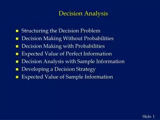
Decision Analysis. A. A. Elimam College of Business San Francisco State University. Characteristics of a Good Decision. Based on Logic Considers all Possible Alternatives Uses all Available Data Applies Quantitative Approach. Decision Analysis Frequently results in a favorable outcome.

E N D
Decision Analysis A. A. Elimam College of Business San Francisco State University
Characteristics of a Good Decision • Based on Logic • Considers all Possible Alternatives • Uses all Available Data • Applies Quantitative Approach Decision Analysis Frequently results in a favorable outcome
Decision Analysis (DA) Steps • Clearly define the problem • List all possible alternatives • Identify possible outcomes • Determine payoff for each alternative/outcome • Select one of the DA models • Apply model to make decision
Types of Decision Making (DM) • DM under Certainty: Select the alternative with the Maximum payoff • DM under Uncertainty: Know nothing about probability • DM under Risk: Only know the probability of occurrence of each outcome
Decision Table Example State of Nature (Market) Alternatives Favorable($) Unfavorable($) -180,000 Large Plant 200,000 -20,000 100,000 Small Plant Do Nothing 0 0
Decision Making Under Risk • Expected Monetary Value (EMV) EMV (Alternative i) = (Payoff of first State of Nature-SN) x (Prob. of first SN) +(Payoff of second SN) x (Prob. of Second SN) +(Payoff of third State of Nature-SN) x (Prob. of third SN) +. . . + (Payoff of last SN) x (Prob. of last SN)
Thompson Lumber Example • EMV(Large F.) = (0.50)($200,000)+(0.5)(-180,000)= $10,000 • EMV(Small F.) = (0.50)($100,000)+(0.5)(-20,000)= $40,000 • EMV(Do Nothing) = (0.50)($0)+(0.5)(0)= $0
Thompson Lumber State of Nature (Market) Alternatives Favorable ($) Unfavorable ($) EMV ($) Large Plant 200,000 -180,000 10,000 100,000 -20,000 Small Plant 40,000 0 0 Do Nothing Probabilities 0.5 0.5
Expected Value of Perfect Information (EVPI) • Expected Value with Perfect Information = (Best Outcome for first SN) x (Prob. of first SN) +(Best Outcome for second SN) x (Prob. of Second SN) + . . . + (Best Outcome for last SN) x (Prob. of last SN)
Expected Value of Perfect Information (EVPI) • EVPI = Expected Outcome with Perfect Information - Expected Outcome without Perfect Information • EVPI = Expected Value with Perfect Information - Maximum EMV
Thompson LumberExpected Value of Perfect Information • Best Outcome For Each SN • Favorable: Large plant, Payoff = $200,000 • Unfavorable: Do Nothing, Payoff = $0 • So Expected Value with Perfect Info. = (0.50)($200,000)+(0.5)(0)= $100,000 • The Max. EMV = $ 40,000 • EVPI = $100,000 - $40,000 = $ 60,000
Decision Table Example Possible Future Demand Alternative Low ($) High ($) 270 Small Facility 200 800 160 Large Facility Do Nothing 0 0
Example A.5 Demand Alternatives Low ($) High ($) EMV ($) 270 Small 200 242 160 800 Large 544 0 0 Do Nothing Probabilities 0.4 0.6
Example A.8Expected Value of Perfect Information • Best Outcome For Each SN • High Demand: Large , Payoff = $800 • Low Demand : Small , Payoff = $200 • So Expected Value with Perfect Info. = (0.60)($800)+(0.4)(200)= $560 • The Max. EMV = $ 544 • EVPI = $ 560 - $ 544 = $ 16
Opportunity Loss : Thompson Lumber State of Nature (Market) Favorable ($) Unfavorable($) 0-(-180,000) 200,000-200,000 0-(-20,000) 200,000-100,000 200,000-0 0 - 0
Opportunity Loss : Thompson Lumber State of Nature (Market) Alternatives Favorable ($) Unfavorable ($) EOL ($) Large Plant 0 180,000 90,000 100,000 20,000 Small Plant 60,000 Do Nothing 200,000 0 100,000 Probabilities 0.5 0.5
Sensitivity Analysis EMV, $ Point 2, p=0.62 EMV(LF) Point 1 p=0.167 200,000 EMV(SF) 100,000 EMV(DN) 0 1 -100,000 Values of P -200,000
Decision Trees • Decision Table: Only Columns-Rows • Columns: State of Nature • Rows: Alternatives- 1 DecisionONLY • For more than one Decision Trees • Decision Trees can handle a sequence of one or more decision(s)
Decision Trees • Two Types of Nodes • Selection Among Alternatives • State of Nature • Branches of the Decision Tree
Decision Tree: Example Favorable (0.5) Large Unfavorable (0.5) F. (0.5) Small U. (0.5) Do Nothing F. (0.5) U. (0.5)
A Decision Tree for Capacity Expansion(Payoff in thousands of dollars) Low demand [0.40] $70 Don’t expand $90 Small expansion High demand [0.60] ($109) 2 Expand 1 ($135) $135 Low demand [0.40] Large expansion ($148) $40 High demand [0.60] ($148) $220
Decision Tree for Retailer Low demand [0.4] $200 High demand [0.6] Small facility Don’t expand ($242) $223 2 Expand $270 ($270) 1 Do nothing $40 Modest response [0.3] 3 ($544) $20 Advertise Low demand [0.4] Large facility ($160) Sizable response [0.7] ($160) $220 High demand [0.6] ($544) $800