Download

1 / 30
300 likes | 341 Views
Decision Analysis. Decision Trees. Any problem that can be presented in a decision table can also be graphically represented in a decision tree Decision trees are most beneficial when a sequence of decisions must be made

E N D
Decision Trees • Any problem that can be presented in a decision table can also be graphically represented in a decision tree • Decision trees are most beneficial when a sequence of decisions must be made • All decision trees contain decision points or nodes and state-of-nature points or nodes • A decision node from which one of several alternatives may be chosen • A state-of-nature node out of which one state of nature will occur
Five Steps toDecision Tree Analysis • Define the problem • Structure or draw the decision tree • Assign probabilities to the states of nature • Estimate payoffs for each possible combination of alternatives and states of nature • Solve the problem by computing expected monetary values (EMVs) for each state of nature node
Structure of Decision Trees • Trees start from left to right • Represent decisions and outcomes in sequential order • Squares represent decision nodes • Circles represent states of nature nodes • Lines or branches connect the decisions nodes and the states of nature
A State-of-Nature Node Favorable Market A Decision Node 1 Unfavorable Market Construct Large Plant Favorable Market Construct Small Plant 2 Unfavorable Market Do Nothing Thompson’s Decision Tree Figure 3.2
EMV for Node 1 = $10,000 = (0.5)($200,000) + (0.5)(–$180,000) Payoffs (0.5) $200,000 Alternative with best EMV is selected (0.5) –$180,000 (0.5) $100,000 (0.5) –$20,000 = (0.5)($100,000) + (0.5)(–$20,000) EMV for Node 2 = $40,000 $0 Thompson’s Decision Tree Favorable Market 1 Unfavorable Market Construct Large Plant Favorable Market Construct Small Plant 2 Unfavorable Market Do Nothing Figure 3.3
Payoffs First Decision Point Second Decision Point Favorable Market (0.78) $190,000 $190,000 2 Unfavorable Market (0.22) –$190,000 –$190,000 Large Plant Favorable Market (0.78) $90,000 $90,000 Small Plant 3 Unfavorable Market (0.22) –$30,000 –$30,000 Survey (0.45) No Plant Results Favorable –$10,000 –$10,000 1 Favorable Market (0.27) 4 Unfavorable Market (0.73) Survey (0.55) Large Plant Results Negative Favorable Market (0.27) Small Plant 5 Conduct Market Survey Unfavorable Market (0.73) No Plant Favorable Market (0.50) $200,000 6 Unfavorable Market (0.50) Do Not Conduct Survey –$180,000 Large Plant Favorable Market (0.50) $100,000 Small Plant 7 Unfavorable Market (0.50) –$20,000 No Plant $0 Thompson’s Complex Decision Tree Figure 3.4
Thompson’s Complex Decision Tree 1. Given favorable survey results, EMV(node 2) = EMV(large plant | positive survey) = (0.78)($190,000) + (0.22)(–$190,000) = $106,400 EMV(node 3) = EMV(small plant | positive survey) = (0.78)($90,000) + (0.22)(–$30,000) = $63,600 EMV for no plant = –$10,000 2. Given negative survey results, EMV(node 4) = EMV(large plant | negative survey) = (0.27)($190,000) + (0.73)(–$190,000) = –$87,400 EMV(node 5) = EMV(small plant | negative survey) = (0.27)($90,000) + (0.73)(–$30,000) = $2,400 EMV for no plant = –$10,000
Thompson’s Complex Decision Tree 3. Compute the expected value of the market survey, EMV(node 1) = EMV(conduct survey) = (0.45)($106,400) + (0.55)($2,400) = $47,880 + $1,320 = $49,200 4. If the market survey is not conducted, EMV(node 6) = EMV(large plant) = (0.50)($200,000) + (0.50)(–$180,000) = $10,000 EMV(node 7) = EMV(small plant) = (0.50)($100,000) + (0.50)(–$20,000) = $40,000 EMV for no plant = $0 5. Best choice is to seek marketing information
Payoffs First Decision Point Second Decision Point $106,400 Favorable Market (0.78) $190,000 $190,000 Unfavorable Market (0.22) –$190,000 –$190,000 Large Plant $63,600 Favorable Market (0.78) $90,000 $90,000 Small Plant $106,400 Unfavorable Market (0.22) –$30,000 –$30,000 Survey (0.45) No Plant Results Favorable –$10,000 –$10,000 –$87,400 Favorable Market (0.27) Unfavorable Market (0.73) Survey (0.55) Large Plant Results Negative $2,400 Favorable Market (0.27) Small Plant $2,400 Conduct Market Survey Unfavorable Market (0.73) No Plant $49,200 $10,000 Favorable Market (0.50) $200,000 Unfavorable Market (0.50) Do Not Conduct Survey –$180,000 Large Plant $40,000 Favorable Market (0.50) $100,000 Small Plant $40,000 Unfavorable Market (0.50) –$20,000 No Plant $0 Thompson’s Complex Decision Tree Figure 3.4
Thompson wants to know the actual value of doing the survey Expected valuewith sampleinformation, assumingno cost to gather it Expected valueof best decisionwithout sampleinformation EVSI = – Expected Value of Sample Information = (EV with sample information + cost) – (EV without sample information) EVSI = ($49,200 + $10,000) – $40,000 = $19,200
Sensitivity Analysis • Sensitivity analysis examines how our decision might change with different input data • For the Thompson Lumber example P = probability of a favorable market (1 – P) = probability of an unfavorable market
Sensitivity Analysis EMV(Large Plant) = $200,000P– $180,000)(1 – P) = $200,000P– $180,000 + $180,000P = $380,000P– $180,000 EMV(Small Plant) = $100,000P– $20,000)(1 – P) = $100,000P– $20,000 + $20,000P = $120,000P– $20,000 EMV(Do Nothing) = $0P + 0(1 – P) = $0
EMV Values $300,000 $200,000 $100,000 0 –$100,000 –$200,000 EMV (large plant) Point 2 EMV (small plant) Point 1 .167 .615 1 Values of P Sensitivity Analysis EMV (do nothing) Figure 3.1
Sensitivity Analysis Point 1: EMV(do nothing) = EMV(small plant) Point 2: EMV(small plant) = EMV(large plant)
EMV Values $300,000 $200,000 $100,000 0 –$100,000 –$200,000 EMV (large plant) Point 2 EMV (small plant) Point 1 EMV (do nothing) .167 .615 1 Values of P Figure 3.1 Sensitivity Analysis
Sensitivity Analysis • How sensitive are the decisions to changes in the probabilities? • How sensitive is our decision to the probability of a favorable survey result? • That is, if the probability of a favorable result (p = .45) where to change, would we make the same decision? • How much could it change before we would make a different decision?
Sensitivity Analysis p = probability of a favorable survey result (1 – p) = probability of a negative survey result EMV(node 1) = ($106,400)p +($2,400)(1 – p) = $104,000p + $2,400 We are indifferent when the EMV of node 1 is the same as the EMV of not conducting the survey, $40,000 $104,000p + $2,400 = $40,000 $104,000p = $37,600 p = $37,600/$104,000 = 0.36
Utility Theory • Monetary value is not always a true indicator of the overall value of the result of a decision • The overall value of a decision is called utility • Rational people make decisions to maximize their utility
$2,000,000 Accept Offer $0 Heads (0.5) Reject Offer Tails (0.5) EMV = $2,500,000 $5,000,000 Utility Theory Figure 3.6
Utility Theory • Utility assessment assigns the worst outcome a utility of 0, and the best outcome, a utility of 1 • A standard gamble is used to determine utility values • When you are indifferent, the utility values are equal Expected utility of alternative 2 = Expected utility of alternative 1 Utility of other outcome = (p)(utility of best outcome, which is 1) + (1 – p)(utility of the worst outcome, which is 0) Utility of other outcome = (p)(1) + (1 – p)(0) = p
(p) Best Outcome Utility = 1 (1 –p) Worst Outcome Utility = 0 Alternative 1 Alternative 2 Other Outcome Utility = ? Standard Gamble Figure 3.7
Investment Example • Jane Dickson wants to construct a utility curve revealing her preference for money between $0 and $10,000 • A utility curve plots the utility value versus the monetary value • An investment in a bank will result in $5,000 • An investment in real estate will result in $0 or $10,000 • Unless there is an 80% chance of getting $10,000 from the real estate deal, Jane would prefer to have her money in the bank • So if p = 0.80, Jane is indifferent between the bank or the real estate investment
p = 0.80 $10,000 U($10,000) = 1.0 (1 –p) = 0.20 $0 U($0.00) = 0.0 Invest in Real Estate Invest in Bank $5,000 U($5,000) = p = 1.0 Investment Example Figure 3.8 Utility for $5,000 = U($5,000) = pU($10,000) + (1 – p)U($0) = (0.8)(1) + (0.2)(0) = 0.8
Investment Example • We can assess other utility values in the same way • For Jane these are Utility for $7,000 = 0.90 Utility for $3,000 = 0.50 • Using the three utilities for different dollar amounts, she can construct a utility curve
Utility as a Decision-Making Criteria • Once a utility curve has been developed it can be used in making decisions • Replace monetary outcomes with utility values • The expected utility is computed instead of the EMV
Utility as a Decision-Making Criteria • Mark Simkin loves to gamble • He plays a game tossing thumbtacks in the air • If the thumbtack lands point up, Mark wins $10,000 • If the thumbtack lands point down, Mark loses $10,000 • Should Mark play the game (alternative 1)?
Tack Lands Point Up (0.45) $10,000 Tack Lands Point Down (0.55) Alternative 1 Mark Plays the Game –$10,000 Alternative 2 Mark Does Not Play the Game $0 Utility as a Decision-Making Criteria Figure 3.11
Utility as a Decision-Making Criteria • Step 1– Define Mark’s utilities U (–$10,000) = 0.05 U ($0) = 0.15 U ($10,000) = 0.30 • Step 2 – Replace monetary values with utility values E(alternative 1: play the game) = (0.45)(0.30) + (0.55)(0.05) = 0.135 + 0.027 = 0.162 E(alternative 2: don’t play the game) = 0.15
Utility Tack Lands Point Up (0.45) E = 0.162 0.30 Tack Lands Point Down (0.55) Alternative 1 Mark Plays the Game 0.05 Alternative 2 Don’t Play 0.15 Utility as a Decision-Making Criteria Figure 3.13