Quality Control of ATLAS II Precipitation Data George J. Huffman 1,2 , Jeremy Lehmann 3,4

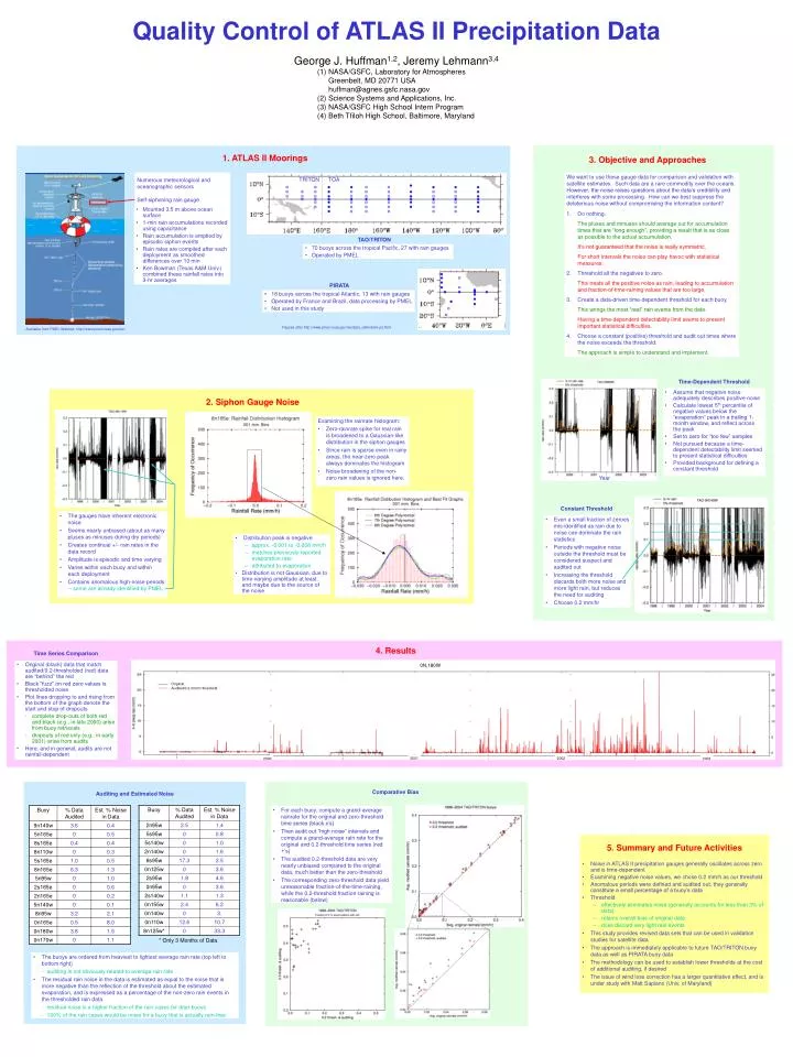
1. TRITON TOA Year 5. Summary and Future Activities • Noise in ATLAS II precipitation gauges generally oscillates across zero and is time-dependent • Examining negative noise values, we chose 0.2 mm/h as our threshold • Anomalous periods were defined and audited out; they generally constitute a small percentage of a buoy’s data • Threshold • effectively eliminates noise (generally accounts for less than 3% of data) • retains overall bias of original data • does discard very light rain events • This study provides revised data sets that can be used in validation studies for satellite data • The approach is immediately applicable to future TAO/TRITON buoy data as well as PIRATA buoy data • The methodology can be used to establish lower thresholds at the cost of additional auditing, if desired • The issue of wind loss correction has a larger quantitative effect, and is under study with Matt Sapiano (Univ. of Maryland) Quality Control of ATLAS II Precipitation Data George J. Huffman1,2, Jeremy Lehmann3,4 (1) NASA/GSFC, Laboratory for Atmospheres Greenbelt, MD 20771 USA huffman@agnes.gsfc.nasa.gov (2) Science Systems and Applications, Inc. (3) NASA/GSFC High School Intern Program (4) Beth Tfiloh High School, Baltimore, Maryland 1. ATLAS II Moorings 3. Objective and Approaches Numerous meteorological and oceanographic sensorsSelf-siphoning rain gauge We want to use these gauge data for comparison and validation with satellite estimates. Such data are a rare commodity over the oceans. However, the noise raises questions about the data’s credibility and interferes with some processing. How can we best suppress the deleterious noise without compromising the information content? • Mounted 3.5 m above ocean surface • 1-min rain accumulations recorded using capacitance • Rain accumulation is emptied by episodic siphon events • Rain rates are compiled after each deployment as smoothed differences over 10 min • Ken Bowman (Texas A&M Univ.) combined these rainfall rates into 3-hr averages Do nothing. The pluses and minuses should average out for accumulation times that are “long enough”, providing a result that is as close as possible to the actual accumulation. It’s not guaranteed that the noise is really symmetric. For short intervals the noise can play havoc with statistical measures. Threshold all the negatives to zero. This treats all the positive noise as rain, leading to accumulation and fraction-of-time-raining values that are too large. Create a data-driven time-dependent threshold for each buoy. This wrings the most “real” rain events from the data. Having a time-dependent detectability limit seems to present important statistical difficulties. Choose a constant (positive) threshold and audit out times where the noise exceeds the threshold. The approach is simple to understand and implement. TAO/TRITON • 70 buoys across the tropical Pacific, 27 with rain gauges • Operated by PMEL PIRATA • 18 buoys across the tropical Atlantic, 13 with rain gauges • Operated by France and Brazil, data processing by PMEL • Not used in this study Figures after http://www.pmel.noaa.gov/tao/data_deliv/deliv-pir.html Available from PMEL Website: http://www.pmel.noaa.gov/tao/ Time-Dependent Threshold • Assume that negative noise adequately describes positive noise • Calculate lowest 5th percentile of negative values below the “evaporation” peak in a trailing 1-month window, and reflect across the peak • Set to zero for “too few” samples • Not pursued because a time-dependent detectability limit seemed to present statistical difficulties • Provided background for defining a constant threshold 2. Siphon Gauge Noise Examining the rainrate histogram: • Zero-rainrate spike for real rain is broadened to a Gaussian-like distribution in the siphon gauges • Since rain is sparse even in rainy areas, the near-zero peak always dominates the histogram • Noise broadening of the non-zero rain values is ignored here. Constant Threshold • The gauges have inherent electronic noise • Seems nearly unbiased (about as many pluses as minuses during dry periods) • Creates continual +/- rain rates in the data record • Amplitude is episodic and time varying • Varies within each buoy and within each deployment • Contains anomalous high-noise periods -- some are already identified by PMEL • Even a small fraction of zeroes mis-identified as rain due to noise can dominate the rain statistics • Periods with negative noise outside the threshold must be considered suspect and audited out • Increasing the threshold discards both more noise and more light rain, but reduces the need for auditing • Choose 0.2 mm/hr • Distribution peak is negative • approx. -0.001 to -0.008 mm/h • matches previously reported evaporation rate • attributed to evaporation • Distribution is not Gaussian, due to time-varying amplitude at least, and maybe due to the source of the noise 4. Results Time Series Comparison • Original (black) data that match audited/0.2-thresholded (red) data are “behind” the red • Black “fuzz” on red zero values is thresholded noise • Plot lines dropping to and rising from the bottom of the graph denote the start and stop of dropouts - complete drop-outs of both red and black (e.g., in late 2000) arise from buoy retrievals - dropouts of red only (e.g., in early 2001) arise from audits • Here, and in general, audits are not rainfall-dependent 0N,180W Original Audited/0.2 mm/hr threshold 2002 2001 2000 2003 Auditing and Estimated Noise Comparative Bias • For each buoy, compute a grand-average rainrate for the original and zero-threshold time series (black x’s) • Then audit out “high noise” intervals and compute a grand-average rain rate for the original and 0.2-threshold time series (red +’s) • The audited 0.2-threshold data are very nearly unbiased compared to the original data, much better than the zero-threshold • The corresponding zero-threshold data yield unreasonable fraction-of-the-time-raining, while the 0.2-threshold fraction raining is reasonable (below) * Only 3 Months of Data • The buoys are ordered from heaviest to lightest average rain rate (top left to bottom right) - auditing is not obviously related to average rain rate • The residual rain noise in the data is estimated as equal to the noise that is more negative than the reflection of the threshold about the estimated evaporation, and is expressed as a percentage of the non-zero rain events in the thresholded rain data - residual noise is a higher fraction of the rain cases for drier buoys - 100% of the rain cases would be noise for a buoy that is actually rain-free