1 / 0

Adding Pictures and Shapes to a Worksheet

Adding Pictures and Shapes to a Worksheet. Lesson 11. Objectives. Software Orientation: The Insert Tab.

qiana
Download Presentation

Adding Pictures and Shapes to a Worksheet

An Image/Link below is provided (as is) to download presentation Download Policy: Content on the Website is provided to you AS IS for your information and personal use and may not be sold / licensed / shared on other websites without getting consent from its author. Content is provided to you AS IS for your information and personal use only. Download presentation by click this link. While downloading, if for some reason you are not able to download a presentation, the publisher may have deleted the file from their server. During download, if you can't get a presentation, the file might be deleted by the publisher.

E N D

Presentation Transcript


  1. Adding Pictures and Shapes to a Worksheet

    Lesson 11
  2. Objectives
  3. Software Orientation: The Insert Tab Microsoft Office includes a gallery of images you can insert into worksheets such as pictures, clip art, shapes, and SmartArt graphics. You can also insert a text box that can be positioned anywhere on the worksheet or insert WordArt to call attention to a worksheet or chart’s primary message. Use the Insert tab (see the figure) to insert illustrations and text. Use this figure as a reference throughout this lesson as you become skilled in inserting and formatting illustrations within a worksheet.
  4. Inserting Pictures While the old adage a picture is worth a thousand words is perhaps an exaggeration, a visual feature adds interest and calls attention to statistical data presented in worksheets. Unlike a worksheet background that is displayed but does not print, pictures, clip art, shapes, and SmartArt graphics are included in worksheet printouts. Graphic objects can be used with charts to focus attention on relevant data.
  5. Inserting a Picture from a File Pictures can be an integral part of creating a compelling worksheet. You can insert or copy pictures into a worksheet from image providers or files on your computer, such as your favorite digital photographs. A well-chosen picture can portray a powerful message, or it can be used to enhance a chart or other Excel graphic display. Using Excel’s Insert Picture command, you can customize the presentation of worksheet data with selected photographs. In the next exercise, you will insert pictures from a file.
  6. Inserting a Picture from a File The manager of Margie’s Travel is preparing a worksheet with detailed travel arrangements for a client’s annual sales meeting to be held at a hotel in Yosemite National Park. The client wants to combine the business travel with a family vacation package. The manager will use your worksheet with photos of the area and add the financial data related to the proposal. The visuals can be formatted to enhance the data and call attention to the most important aspects of the workbook.
  7. Step-by-Step: Insert a Picture from a File Before you begin these steps, LAUNCH Microsoft Excel and create a new Blank workbook. Click the Sheet1 tab. Click Format in the Cells group on the Home tab and click Rename Sheet from the drop-down menu that appears. Key Vernal Fall to replace the selected Sheet1 text, and press Enter. Use the same process to rename Sheet2 to El Capitan and to rename Sheet3 to Sequoias. Select A1 on the Vernal Fall worksheet. On the Insert tab, click Picture. The Insert Picture dialog box opens.
  8. Step-by-Step: Insert a Picture from a File In the dialog box directory, navigate to the data files for this lesson, and then click Vernal Fall. Click Insert. The picture is inserted and, as shown in the figure, the Format tab with Picture Tools is added to the Ribbon. Select the number in the Shape Height text box, key 5, and press Enter. The image changes to a height of 5 inches, with its width automatically proportioned.
  9. Step-by-Step: Insert a Picture from a File Select A1 on the El Capitan worksheet. Click the Insert tab and click Picture. In the Insert Picture dialog box, navigate to the data files for this lesson and click the El Capitan image, then click Insert. The picture is inserted and the Picture Tools become available. Select the Shape Height value, key 5, and press Enter. Select A1 on the Sequoias worksheet. Click the Insert tab and click Picture. In the dialog box, click Sequoias to select it from the data files. Click Insert to insert the picture. Select the Shape Height value, key 5, and press Enter. Create a Lesson 11 folder and SAVE as Yosemite. LEAVE the workbook open to use in the next exercise.
  10. Inserting a Clip Art Picture A clip refers to a single media file including art, sound, animation, or movies. A clip art image is a single piece of readymade art, often appearing as a bitmap or a combination of drawn shapes. You can insert a clip art image into a worksheet from Microsoft Office Online, other image providers, or files on your computer. When you search for clip art in Excel, your search results can include clip art, photographs, movies, and sound files. In the next exercise, you will insert clip art into your worksheet.
  11. Inserting a Clip Art Picture The professional-quality photos returned by a clip art search are usually more appropriate in a business document than caricature-type artistic designs. Some of the photos in the clip art gallery have been sized to easily insert into a document, and you do not always need to adjust the size, as you did in the first exercise, to easily view the picture. If you frequently use illustrations in your worksheets, you can organize your favorites in the Microsoft Clip Organizer. The Clip Organizer is a way to gather and store your own clips so that you can easily locate and insert them into documents. You can access the Clip Organizer from the Clip Art task pane.
  12. Inserting a Clip Art Picture The first time you open the Clip Organizer, you are asked if you want the organizer to scan your computer for photos and other media files and organize them into separate collections. Clip Organizer creates a shortcut to the files in their original location; it does not copy or move the files on your computer. The shortcuts let you preview, open, or insert a media file without going to its installed location. You can let the Clip Organizer decide which folders and hardware drives to scan for files, or you can specify where to search.
  13. Inserting a Clip Art Picture The folders in the Clip Organizer have the same names as the folders in which the original files are stored. Clip Organizer automatically adds keywords to media files. You can modify, delete, or add new keywords to ensure that you will find the clip when you want to insert it into a document. When you download or copy files from a clip art source such as Microsoft Online, the image will be stored in the Clip Organizer. Clips organized and saved in Excel can then be used in Microsoft Word and PowerPoint documents and on the Margie’s Travel Website.
  14. Step-by-Step: Insert a Clip Art Picture USE the workbook from the previous exercise. Click on any blank cell in the Sequoia worksheet. On the Home tab, click Insert and click Insert Sheet. Click the rename option in the Cells group, and then click Insert Sheet from the drop-down menu that appears. Click to select the text in the new worksheet’s tab, and then rename the sheet Clip Art. On the Insert tab, click Clip Art. The Clip Art task pane opens on the right side of the Excel window.
  15. Step-by-Step: Insert a Clip Art Picture Click the Results should bedrop-down arrow and place a check mark in all media types. In the Searchfor field, key waterfall and click Go. Results are displayed similar to those shown in the figure. Your results will return more than just graphics. Be sure not to select any audio or video file. Click any image in the search results to insert a waterfall into the Clip Art worksheet.
  16. Step-by-Step: Insert a Clip Art Picture In the Clip Art task pane, click the arrow in the Resultsshould be field. Deselect all media types except Illustrations (as shown in the figure). Click Go. The results include only clip art images. Scroll through the list and click an image to insert a waterfall clip art image. SAVE and CLOSE the workbook. CLOSE the Clip Art task pane. LEAVE Excel open to use in the next exercise.
  17. Using SmartArt Graphics A SmartArt graphic is a visual representation of information and ideas. SmartArt graphics can be used with other images and decorative text. When you insert a SmartArt image into your worksheet, the Text pane should appear to the left of a SmartArt graphic, containing bullets that represent the shapes in the graphic. The Text pane works like an outline or a bulleted list that maps information directly to the graphic. You can use the pane to enter and edit the text that appears in the graphic.
  18. Using SmartArt Graphics SmartArt should not be confused with clip art. Clip art is an actual image. SmartArt is a graphical representation of something other than an image that you would want to add to a worksheet. An example would be a flowchart. The SmartArt library has many different styles and themes that can be applied to the worksheet. You can build the flowchart, add text to it, change its appearance, move the objects on the worksheet, and make it ready for presentation. In the next exercise, you will apply SmartArt graphics.
  19. Using SmartArt Graphics When choosing a layout for a SmartArt graphic, determine what you want to convey and how your information should appear, then try different layouts until you find the one that best illustrates your message. Your graphic should be clear and easy to follow. Single descriptive words and short descriptive phrases are recommended for your graphic. The table lists the seven types of SmartArtgraphics and a short description of the purpose of each type.
  20. Using SmartArt Graphics If you cannot find the exact layout that you want, you can add and remove shapes in your SmartArt graphic to adjust the structure of the layout. When you add or remove shapes and edit the text, the arrangement of the shapes and the amount of text within those shapes is updated automatically. The original design and border of the layout is maintained. Although you cannot drag text into the Text pane, you can copy and paste to the pane. Also, you can copy from the Text pane to any Microsoft Office program.
  21. Using SmartArt Graphics When you click away from the SmartArt graphic, the Text pane disappears. You can show or hide the Text pane by clicking the control on the left side of the SmartArt graphic or by clicking Text Pane on the Design tab. In general, SmartArt graphics work best with small amounts of text. Larger amounts of text detract from the visual appeal of the graphic and make it more difficult to convey your message visually.
  22. Step-by-Step: Use SmartArt Graphics OPEN the Cruise Dates file for this lesson. On the Mexico worksheet, select C24. On the Insert tab, in the Illustrations group, click SmartArt. The Choose a SmartArt Graphicdialog box is displayed as shown in the figure.
  23. Step-by-Step: Use SmartArt Graphics In the Choose a SmartArt Graphic dialog box, click Cycle in the type pane on the left side of the dialog box. Click Block Cycle (top row, third from left) in the layout pane on the right side of the dialog box. Click OK. The Cycle graphic image is inserted and SmartArt Tools are available on the Design and Format tabs. When it is inserted, the graphic is joined by its Text pane. This pane allows the user to enter the information to be contained in the SmartArt graphic.
  24. Step-by-Step: Use SmartArt Graphics On the Design tab, shown in the figure, click the Text Pane button in the Create Graphic group if the Text pane is not displayed when the graphic is inserted. Point to the Block Cycle layout name at the bottom of the Text Pane to see a ScreenTip; holding a description of the best use for the selected SmartArt layout.
  25. Step-by-Step: Use SmartArt Graphics The Text pane and the SmartArtgraphic have placeholder text that you can replace with your information. The first Text placeholder will be selected as shown in the figure. Key May 20. As you key text in the Text pane, it is displayed in the first block of the Cycle graphic.
  26. Step-by-Step: Use SmartArt Graphics Click, hold, and drag the SmartArt graphic to rest below the cells in the worksheet. Select E5 in the data range and click Copy. Click the graphic, select the second [Text] placeholder, and click Paste. The date of June 17 that you copied has now been pasted into the second graphic. Copy E6 and paste the date in the third [Text] placeholder. Copy the text in E7 to the fourth [Text] placeholder. Copy the text in E8 to the last [Text] placeholder. Press Enter to add an additional text placeholder and an additional block to the Cycle graphic.
  27. Step-by-Step: Use SmartArt Graphics Copy the text in E9 to the last block. Click outside the image to view the Cycle graphic image as it is displayed in the worksheet. The text pane is hidden from view and only the graphic with its formatting remains. The deselected graphic is shown in the figure. Refer to the previous screen for the graphic with its text pane. SAVE the workbook as Cruise 1. LEAVE the workbook open to use in the next exercise.
  28. Adding Shapes You can add a shape to a workbook or combine multiple shapes to create a drawing or a more complex shape. Available shapes include lines, basic geometric shapes, arrows, equation shapes, flowchart shapes, stars, banners, and callouts.
  29. Inserting Basic Shapes You can use a shape to call attention to an important aspect of worksheet data. Excel provides a variety of basic shapes that you can insert. You can add shapes to a chart or on top of a SmartArt graphic to customize the chart or SmartArt graphic. When you use more than one shape, it does not matter which shape you insert first. You can use the Bring to Front and Send to Back commands to place the shape containing text on top so that the text is visible. In the next exercise, you insert and format basic shapes in Excel, and place one shape on top of another to achieve a desired result.
  30. Step-by-Step: Insert Basic Shapes USE the workbook from the previous exercise. On the Alaska worksheet, click A5. Click Shapes in the Illustrations group on the Insert tab. The Shapes gallery shown in the figure opens. Click Rounded Rectanglein the Rectangles group in the Shapes gallery and click A5 to place the rectangle in that cell. Use the rectangle’s handles to resize it to hide the text in row 5 from A5 to the right boundary of F5 of the worksheet.
  31. Step-by-Step: Insert Basic Shapes On the Format tab, in the Shape Styles group, click Colored Outline – Orange, Accent 6 (first outline style). This places the colored border around the graphic. Click Shape Fill in the Shape Styles group and click No Fill. Click an empty cell to deselect the rectangle. The cell’s text is now visible since you chose the no fill option. The colored outline shape calls attention to the Southbound Glacier Discovery cruise that leaves Seattle on June 4. Click WordArt in the Text group on the Insert tab. In the WordArt gallery, click Fill – Orange, Accent 6 Outline – Accent 6, Glow – Accent 6 (second row, second style). The WordArt sample text Your Text Here is placed.
  32. Step-by-Step: Insert Basic Shapes Click the Home tab, place your insertion point in the number in the Font Size box and key 36. Press Enter. The Your text here text is still selected; replace it by keying Lowest Price of the Summer in the WordArt text box. Move the WordArt text box so that it is several rows directly below the last row of data and aligned with the data range. On the Insert tab, click Shapes and click Double Arrow (third option from the left) in the Lines group. Click C5 to position the arrow from C5 to the WordArt below the data range (see the figure).
  33. Step-by-Step: Insert Basic Shapes Click the Insert tab. On the Mexico worksheet, click Shapes. In the Rectangles group, click Snip Same Side Corner Rectangle (fourth from left) in the Rectangles section of the gallery. Click in the center of the existing SmartArt to place the new shape. Click Colored Outline – Orange, Accent 6 in the Shape Styles group. Use the shape’s handles to resize the rectangle and drag the rectangle to cover the SmartArt graphic. Click Send Backward in the Arrange group on the Format tab. SAVE your workbook. LEAVE the workbook open to use in the next exercise.
  34. Drawing Lines You may want to add a line to point to data in a specific location, create a signature line, or separate text. A connector is a line that has connection points at the ends of the line and stays connected to the shape to which you have connected it. Straight, elbow, and curved lines are available. In the next exercise, you add two text boxes to your worksheet, and then insert connector lines to connect the text boxes.
  35. Drawing Lines When you rearrange shapes that are joined by connectors, the connectors move with the shapes. You can move the end of a connector to detach it from the shape. You can then attach it to another connection site on the same shape, attach it to another shape, or delete the connector. When you select the connector, you can click the diamond shape in the center of the connector and change the angle of the connector line.
  36. Drawing Lines If you want to draw a line without connection points, click Freeform in the Shapes gallery. Click one position in the document, move your pointer to a different location, and click again. When you are finished drawing the line, double-click. If you attach shapes with a line without arrow points, you can add an arrowhead to the line after it has been attached to a shape. Under Drawing Tools on the Format tab, click the arrow next to Shape Outline and point to Arrows. Click the arrow style you want.
  37. Step-by-Step: Draw Lines USE the workbook from the previous exercise. On the Advertising worksheet, on the Insert tab, in the Text group, click Text Box. Select A2 and draw a text box that covers A2:A4. Your cursor will become an upside-down cross when you have chosen the text box option. You simply point to the place where you want to start the box, click, hold, and drag to the area of the worksheet where you want the text box to end and then release the mouse. It might take several tries before you get used to the process (see the figure).
  38. Step-by-Step: Draw Lines Click inside the box and then key Cruise in the text box. Click the Insert tab. Click Text Box and select C5. As in step 2, draw a text box that covers C5:C7. Key Relax in the text box. Click the Insert tab. Click Text Box and select E8. Draw a text box that covers E8:E10. Key Enjoy in the text box. On the Insert tab, click Shapes in the Illustrations group. In the Lines section of the gallery, click Elbow Double-Arrow Connector (sixth from the left). Red circular dots (the connection points) appear on the text boxes as you move your pointer over them.
  39. Step-by-Step: Draw Lines Click on the Cruise textbox to reveal the connection points. Black indicators show where you can attach a connector. Click the right connection point on the Cruise text box and drag the connection arrow to the left connection point on the Relax text box. Use the same procedure in step 8 to connect the Relax text box to the Enjoy text box. Your worksheet should look like the figure.
  40. Step-by-Step: Draw Lines Click the border of the Cruise text box to display the move arrow. Drag the box to A8. The connection line remains with the text box. Move the Cruise text box to A2:A4. SAVE your workbook. LEAVE the workbook open to use in the next exercise. NOTE: After you have connected the text boxes, you can move the connection line independently, but not the boxes that the connector links.
  41. Inserting a Block Arrow Insert block arrows when you want to show steps in a process or show a timeline. You can insert a block arrow from the Shapes gallery, or you can insert a SmartArt graphic and select the Continuous Arrow Process. The SmartArt Continuous Arrow Process arrow is used to show a timeline or sequential steps in a task, process, or workflow. The standard block arrow can serve the same purpose or be used to call attention to data in the worksheet. In the next exercise, you will insert block arrows into the worksheet.
  42. Step-by-Step: Insert a Block Arrow USE the workbook from the previous exercise. On the Hawaii worksheet, click the Insert tab if necessary and then click Shapes. Under Block Arrows, click Right Arrow. Move the insertion crosshairs to A11 and drag the block so that the arrow point touches the right corner boundary of B12. The arrow will remain selected. Key Explore the Islands!. On the Insert tab, click SmartArt, and click Process in the SmartArt type pane.
  43. Step-by-Step: Insert a Block Arrow Click Continuous Arrow Process (third row, third from left) and click OK. See the figure. Click any edge of the SmartArt image to display the move pointer and click and drag the pointer to move the image below the block arrow shape.
  44. Step-by-Step: Insert a Block Arrow The first placeholder is already active. Key Call Today!. In the second placeholder, key Sail this Summer!. Select the third [Text] placeholder and press Backspace to delete the third placeholder bullet. SAVE and CLOSE the workbook. LEAVE Excel open to use in the next exercise.
  45. Creating a Flowchart A flowchart is a schematic representation of a process—a working map for reaching your final product or decision. A flowchart shows the steps in a process, such as in the instructions for assembling a new computer, a diagram of a manufacturing plant’s work flow, or the required steps for responding to a request for proposal (RFP). You can create a flowchart by inserting Flowchart shapes and connectors or use a Process SmartArt graphic. You can add more detail when you create a flowchart by using the flowchart shapes. The SmartArt graphic saves time but provides less detail.
  46. Creating a Flowchart The flowchart’s intended use and the amount of detail needed determine which style should be used. In the next exercise, you construct a flowchart. Flowchart shapes provide an indication of what happens during the flow of work. In the Flowchart worksheet, for example, the chart begins with a Preparation shape. Use a diamond shape to indicate a decision. Connector arrows point one direction if the decision is no, and point the other direction for yes. See the figure.
  47. Step-by-Step: Create a Flowchart OPEN the Graphics workbook file for this lesson. On the Flowchart 1 worksheet, click the Insert tab, and then click Shapes to produce the Shapes gallery. In the Block Arrows section of the gallery, click Down Arrow. The arrow is now in the work-sheet. Move the newly inserted arrow to the bottom point of the last diamond. Adjust the arrow’s size to resemble the arrows. Move to have the arrow reside below the point of the diamond (see the figure).
  48. Step-by-Step: Create a Flowchart Click the Insert tab and click Shapes. In the Shapes gallery, click the Flowchart: Process shape. Insert the image below the arrow. Make the newly inserted arrow the approximate size of the existing arrows. Click in the Process shape, then key Prepare worksheet to calculate potential earnings. Click Sheet2 and rename it Flowchart 2. With the Flowchart 2 worksheet the active sheet, click the Insert tab, and click SmartArt. The Choose a SmartArt Graphic dialog box opens.
  49. Step-by-Step: Create a Flowchart Click Process in the Type pane. Scroll through the list, pointing to the process to locate and click Vertical Process (sixth row, third from left) in the Layout pane. The Vertical Process layout is used to show a progression or sequential steps in a task, process, or work flow from top to bottom. This SmartArt layout works best with Level 1 text without a great deal of detail. Click OK to insert the graphic. The SmartArt Tools tab is now active on the Ribbon. With the insertion point in the first [Text] placeholder in the Text pane, key Review RFP. In the second placeholder, key Personnel?.
  50. Step-by-Step: Create a Flowchart In the third placeholder text box, key Time?. Press Enter. You have now added another text box in the text pane. Key Prepare Worksheet. The size and shape of the rectangles in the diagram change as you enter a longer text string. SAVE the workbook as Graphics 1. LEAVE the workbook open to use in the next exercise.
  51. Creating an Organization Chart One of the most common uses for the Hierarchy layout is a company organization chart. An organization chart graphically illustrates the management structure of an organization. When you choose this layout, additional functionality, such as the assistant shape and hanging layouts, become available. In the next exercise, you will create and modify an organization chart.
  52. Step-by-Step: Create an Organization Chart USE the workbook you saved in the previous exercise. Click the Sheet3 tab. Right-click, click Format, click Rename Sheet; the Sheet3 text in the worksheet tab is selected. Key Organization Chart and press Enter. On the Insert tab, click SmartArt to open the Choose a SmartArt Graphic dialog box. Click Hierarchy in the Shape Type pane. Click Organization Chart in the layout pane and click OK. In the first [Text] placeholder, key Margie Shoop, CEO, and press Enter. You have added a new text placeholder.
  53. Step-by-Step: Create an Organization Chart Click Demote in the Create Graphic group on the Design tab to demote the box to Level 2. This moves the box one level below the CEO and to the left. Key John Y. Chen and press Enter. You have now added another Text placeholder. Click Demote and key Jamie Reding. Press Enter. This new text placeholder is now one level below John Y. Chen. Key Stephanie Conway and press Enter. You have now created another text placeholder. Click Promote and key Ciam Sawyer. Press Enter. You have now created another text placeholder.
  54. Step-by-Step: Create an Organization Chart Click Demote and key Jeffrey Ford. This now moves the text placeholder one level below Ciam Sawyer. Click inside the text of the first text placeholder (Margie Shoop, CEO) in the Text pane, then click the drop-down list arrow next to Add Shape in the Create Graphic group on SmartArt Tools Design tab. The Add Shape drop-down list appears. Click Add Assistant in the drop-down list that appears. Key Brenda Diaz, Assistant in the new text placeholder that appears in Text pane.
  55. Step-by-Step: Create an Organization Chart Select any blank placeholders in the Text pane and click Delete. If necessary, press Backspace to delete the last blank text placeholder. Move the graphic to the upper left corner of the worksheet. Click outside the graphic. Your organization chart should look like the figure. SAVE your workbook. LEAVE the workbook open to use in the next exercise.
  56. Copying or Moving a Graphic Pictures, clip art, shapes, and SmartArt graphics are not always inserted where you want them for an effective presentation. You can move a graphic manually, or specify its exact size by using options in the Size group on the Format tab. When you want to move a graphic incrementally, use the arrow keys, which provide precision. Click the graphic border and move the graphic for a significant change in location.
  57. Copying or Moving a Graphic You can copy a SmartArt graphic, or any other graphical display, and paste it to another location within the worksheet, paste it to another worksheet or workbook, or paste it to another Microsoft Office program. You can move a shape in a SmartArt graphic, or you can move the whole graphic. This flexibility allows you to customize the design of the graphical display. In the next exercise, you will move and copy graphics.
  58. Step-by-Step: Copy or Move a Graphic USE the workbook you saved in the previous exercise. Click the Flowchart 2 tab to open the worksheet. Click the SmartArt graphic to select it. Press the up, down, left, or right directional arrows on your keyboard to move the graphic so that it fills F4:H18. Click anywhere in the Flowchart 2 graphic. Click Copy on the Home tab to copy the graphic Click the Flowchart 1 worksheet, select D32, and click Paste; the graphic appears in cell D32.
  59. Step-by-Step: Copy or Move a Graphic Click the right-center border of the graphic and drag the border to the right boundary of column M. Click the first rectangle (Review RFP) in the organization chart and drag it to the left and down so that it is parallel to the second rectangle (Personnel?). Notice that the arrow now points to the right towards the other rectangle. SAVE the workbook. LEAVE the workbook open to use in the next exercise.
  60. Formatting Graphics The formatting styles such as font, fill color, and effects that are applied when you insert a shape or SmartArt graphic are based on the underlying document theme of the worksheet. You can apply a Quick Style to an entire graphic or apply formatting components to various parts of a graphic.
  61. Applying Styles to Shapes Quick Styles are combinations of different formatting options. They are displayed in a thumbnail in various Quick Style galleries on the Format tab that is added to the Ribbon when a graphic is inserted in a worksheet. When you place your pointer over a style thumbnail on the Format tab, you can see how applying that style will affect your SmartArt graphic or shape. In the next exercise, you change the appearance of a graphic by applying formatting to flowchart components to preview various formatting styles.
  62. Applying Styles to Shapes After trying several effects, you can select a basic style to use throughout the flowchart rather than have such varying styles in one graphic. In the next exercise, you will be applying shape styles to the SmartArt. To prevent the formatting of a graphic from overpowering the message, apply formatting sparingly. When a graphic is composed of individual shapes, you must select the shapes to which you want to apply formatting.
  63. Step-by-Step: Apply Styles to Shapes USE the workbook from the previous exercise. On the Flowchart 1 worksheet, at the top of the Organization chart, select the Start shape. The Drawing Tools tab is now active on the Ribbon. Click the Format tab and click the more arrow next to the predefined Outline Styles in the Shape Styles group. This opens the Outline Colors gallery. In row 4, click Subtle Effect – Red, Accent 2. You have now applied this style to the Start object.
  64. Step-by-Step: Apply Styles to Shapes Select the first diamond shape, press Shift, and select the second diamond. You have now selected both objects. Click Shape Fill and click Red, Accent 2. With the shapes still selected, click Shape Outline. Click Dash Dot. Click Shape Effects, point to Glow, and click the first option (Blue 5 pt. glow, Accent color 1) in the Glow gallery.
  65. Step-by-Step: Apply Styles to Shapes Click Text Fill in the WordArt Styles group and click Dark Blue in standard colors. You have changed the shape text as illustrated in the figure. SAVE the workbook. LEAVE the workbook open to use in the next exercise.
  66. Applying Quick Styles to Graphics SmartArt styles reflect the document theme that was chosen when the worksheet was created. You can apply a different style from those displayed on the Design tab, or you can modify elements within the graphic by changing the shape fill, outline, or effects. You can point to a style and see how that style will look in your display, rather than applying and undoing numerous styles in order to find the one you want to use. That way, you can see the effect without changing anything on your worksheet. In the next exercise, you will format shapes by applying quick styles.
  67. Step-by-Step: Apply Quick Styles to Graphics USE the workbook from the previous exercise. On the Flowchart 2 worksheet, select the SmartArt graphic. Click the Design tab. In the SmartArt Styles group, the style that is currently applied to the graphic, based on the Office theme, is selected. The style choices that are available in the SmartArt Styles group on the Design tab are based on the colors, fonts, and effects that comprise the Office theme. Point to each style that is displayed to see the changes that applying the style would have on the SmartArt graphic. Click White Outline.
  68. Step-by-Step: Apply Quick Styles to Graphics Click the more arrow in the bottom right corner of Smart Art styles and point to various styles in the Best Match for Document list to observe changes to the graphic. Preview the styles in the 3-D group and click Metallic Scene (third row, first option on left). When you change the worksheet’s theme, the options in the styles gallery change to reflect the new theme that you have applied to the worksheet.
  69. Step-by-Step: Apply Quick Styles to Graphics Click Change Colors and click Colorful – Accent Colors. The choices in the SmartArt Styles group have changed based on changing the graphics colors. When you insert a SmartArt graphic, a color diagram of the style you select is displayed on the Choose a SmartArt Graphic dialog box. The color combination displayed in that sample was applied to the graphic when you clicked Change Colors. On the Organization Chart worksheet, click the SmartArt graphic. Click Subtle Effect in the SmartArt Quick styles window in the SmartArt Styles group. SAVE the workbook as Graphics 2. LEAVE the workbook open to use in the next exercise.
  70. Resizing a Graphic You can resize one or more shapes within a graphic or resize the complete SmartArt graphic. You can use the sizing handles on the side or corner of a graphic to increase or decrease its size, or you can specify a specific size for the height and width of a graphic or shape within the graphic. In the next exercise, you will learn how to resize the graphic using the sizing tools on the Ribbon.
  71. Step-by-Step: Resize a Graphic USE the workbook from the previous exercise. On the Organization Chart worksheet, click in the SmartArt graphic to select it. Click the left-center sizing handle and drag it to the column G right boundary. On the Format tab, click Size. In the Height box, key 5.5. In the Width box, key 6. You have now resized the shape. Click the shape at the top of the diagram (Margie Shoop, CEO). Click the right sizing handle and drag to the right until the shape extends over the rest of the chart. SAVE and CLOSE the workbook. LEAVE Excel open to use in the next exercise.
  72. Rotating a Graphic You can change a shape’s position by rotating or reversing it. Reversing a shape is also referred to as creating a mirror image or flipping. When you rotate multiple shapes, they are not rotated as a group, but each shape is rotated around its own center. The predefined rotation options limit you to flipping the graphic. When you open the Size and Properties dialog box, you can rotate a graphic one degree at a time, which gives you a great deal of flexibility in placing the graphic at exactly the angle that calls attention to the most significant data in a worksheet. In the next exercise, you will learn to reposition by rotating the shape.
  73. Step-by-Step: Rotate a Graphic OPEN the Take a Summer Cruise file for this lesson. On the Hawaii worksheet, select the text in the standard block arrow (Explore the Islands!). Key Pick a Cruise!. Click the Format tab. In the Arrange group, click Rotate and click FlipHorizontal. The arrow is reversed. The text will remain facing in the original direction. Click Rotate and click RotateRight90º. The arrow is now pointing up. Mouse over the graphic, displaying the move pointer, and move it so that the arrow tip is centered in the whitespace in A6.
  74. Step-by-Step: Rotate a Graphic Click the SmartArt graphic. On the Design tab, click RighttoLeft in the Create Graphics group. The graphic is reversed horizontally. The text also moved in correspondence with the movement of the arrow. On the Format tab, click Arrange, and then click SelectionPane. On the Selection and Visibility pane, click RightArrow1. On the Format tab, click Rotate and then click MoreRotationOptions. The Format Shape dialog box is displayed with the Size options showing. On the Size and rotate area, click the downarrow in the Rotation field until the graphic rotation is 70º. Click Close.
  75. Step-by-Step: Rotate a Graphic Move the graphic so that all text is visible and the point is centered in the white space in A6 as illustrated in the figure. Close the SelectionandVisibility pane. Also, on the Page Layout tab, in the Sheet Options group, deselect the worksheet Gridlines so they no longer display in the worksheet. SAVE the workbook as Cruise 2. LEAVE the workbook open to use in the next exercise.
  76. Resetting a Picture to Its Original State Sometimes you make formatting changes and then want to restore a picture or graphic to its original formatting. The Reset Picture command on the Picture Tools Format tab will reset picture formatting to the formatting present when the file was last saved. In the next exercise, you will manipulate picture settings and then reset them back to their original state.
  77. Step-by-Step: Reset a Picture to Its Original State USE the workbook from the previous exercise. On the Mexico worksheet, select the picture. The Picture Tools tab is now active. Click the Format tab. Click the Crop icon. On the drop-down list, click Crop to Shape and then in the Rectangles options, choose Snip Same Side Corner Rectangle. This crops the right and left top corners of the picture.
  78. Step-by-Step: Reset a Picture to Its Original State In the Picture Quick Styles window, in Picture Styles group, click Metal Frame (3rd style). The corners of the picture have now reappeared and there is a metal frame border in place. Click the Corrections button in the Adjust group the corrections drop-down list opens. In the Brightness and Contrast area, click Brightness: +20% Contrast: –40% (4th option in first row). You have now adjusted the brightness and contrast of the picture.
  79. Step-by-Step: Reset a Picture to Its Original State In the Adjust group, click the Color button. The Color drop-down list opens. On the list, in the Recolor section, click Dark Blue, Text color 2 Dark. You have now changed the image to reflect the applied colors (see the figure). Click Reset Picture in the Adjust group. SAVE the workbook with the same name and CLOSE. LEAVE Excel open for the next exercise.
  80. Adding Graphic Enhancements Using Picture Tools New to Office 2010 are enhanced photo editing capabilities. Along with the inclusion of Live Preview, this gives the application user the opportunity to create vibrant, stylistic, and professional picture edits without the need for a third-party program or add-in. Upon selection of your graphic, the picture tools are activated on the Ribbon. In the next section, you will be applying artistic effects, color features, picture effects, corrections, borders, and managing picture properties.
  81. Changing a Graphic with Artistic Effects Located in the Adjust Group on the Ribbon, you will find the button for Artistic Effects. This new feature allows you to edit images to apply effects such as marker, crisscross etching, photocopy, pastels smooth, and glow edges, to list a few. The Artistic Effects feature allows for a more dynamic use of images in workbooks and worksheets. In the next exercise, you will choose and apply several artistic effects to images.
  82. Step-by-Step: Change a Graphic with Artistic Effects Before you begin these steps, LAUNCH Microsoft Excel and create a new Blank workbook. Click on the Insert tab. Choose the Skyline image from the Lesson 11 folder. The image is now inserted into the worksheet. Move the image to align with cell B11. Under Picture tools, on the Format tab, in the Adjust group, click the Artistic Effects button, shown in the figure.
  83. Step-by-Step: Change a Graphic with Artistic Effects Mouse over the effects’ thumbnails in the gallery. Note that your Live Preview shows you what your changes will look like. Click on Cutout. You have now applied the artistic effect. SAVE the workbook as Skyline 11 in the Lesson 11 folder. CLOSE the workbook. LEAVE Excel open for the next exercise. NOTE: If you compress a picture to reduce its size, the amount of detail retained in the image will change, making the image look different than before it was compressed. To avoid this, compress it before applying an artistic effect. You can recompress the file after you save your effects as long as you have not closed the program you are working in.
  84. Using the Color Feature to Enhance Images The Color tool is located in the Adjust group on the Ribbon. It allows you to apply changes and color to the image you are using. All these enhancements change the output and look of the picture, altering it from its original state. In this next exercise, you will use the Color tools to apply different colors to the picture and you will apply these photo enhancements—saturation, tone, contrast, and recolor.
  85. Step-by-Step: Use the Color Feature Before you begin these steps, LAUNCH Microsoft Excel and create a new Blank workbook. Click on the Insert tab. Choose the Vintage Car image from the student data files for this lesson. Move the image to align with cell B11. Under Picture tools, on the Format tab, within the Adjust group, click the Color button; the color gallery opens (see the figure on slide 87).
  86. Step-by-Step: Use the Color Feature In the Color Saturation section, mouse over the Saturation 33% thumbnail. You will see the picture change in the worksheet with Live Preview. Click on the thumbnail to apply the change. The picture has now changed on the worksheet. Click the Color button in the Adjust group; the Color gallery opens. In the Color Tone section, mouse over the Temperature: 7200 K thumbnail. Click to apply. The image has now changed again to apply the new color style.
  87. Step-by-Step: Use the Color Feature Click the Color button in the Adjust group; the Color gallery opens. In the Recolor section, mouse over several of the thumbnails and note the changes to your image in the workbook. Click on the Orange, Accent color 6 Light. Your image has now had the settings applied as illustrated in the figure. SAVE the workbook as Antique Auto in the Lesson 11 folder. LEAVE the workbook open for the next exercise.
  88. Making Corrections to a Graphic The Corrections button is located in the Adjust group on the Ribbon. The Corrections tool allows you to adjust an image’s brightness and contrast, and sharpness and softness. In the next exercise, you will use the Corrections tools to apply these corrections.
  89. Step-by-Step: Make Corrections to a Graphic USE the workbook from the previous exercise. With the image and the Format tab active, click on the Corrections button, in the Adjust group, to produce the Corrections option gallery, as seen in the figure.
  90. Step-by-Step: Make Corrections to a Graphic In the Sharpen and Soften section, choose and apply Soften: 50%. This setting will apply these changes to the picture and change its overall look. Click the Corrections button. In the Brightness and Contrast section, choose and apply Brightness: +20% Contrast: –40%. This setting will apply these changes to the picture and change its overall look. These changes do not overwrite the previous step but are included with them. SAVE the workbook as Edited Vintage Auto. LEAVE workbook open for the next exercise.
  91. Applying a Picture Style There are 28 built-in picture styles in Excel’s Picture group. With the new Live Preview feature in Office 2010, you can simply mouse over the style of your choice and view the change on your screen before choosing and applying your style. In the next exercise, you will apply Picture styles to the graphic.
  92. Step-by-Step: Apply a Picture Style USE the workbook from the previous exercise. Click the drop-down arrow in the Picture Styles group to open the Picture Styles thumbnail galley, as shown in the figure. Mouse over several of the styles and note the changes with Live Preview. Click to apply Snip Diagonal Corner, White. SAVE the changes as Vintage Auto Style. CLOSE the workbook. LEAVE Excel open for the next exercise.
  93. Customizing Picture Borders Once you have applied a picture style, you can modify and customize it. Besides the built-in presets, you can apply such enhancements as shadow, reflection, glow, soft edges, bevel, and 3-D rotation. Once again, the Live Preview feature allows you to view your choice onscreen before you choose and apply it to your image. You will enhance your pictures in this next exercise with picture borders.
  94. Step-by-Step: Customize Picture Borders OPEN the previously created Skyline 11 file from the Lesson 11 folder to use with this exercise. Click on the image to make it active. Click the Format tab. Click the Picture Border command, in the Theme Colors gallery, choose and apply Red, Accent 2, Lighter 40%. The red border is now placed around the picture. Click on any empty cell to deselect the picture and view the border.
  95. Step-by-Step: Customize Picture Borders Click on the Picture Border command, point to Weight. From the Line Weight drop-down list, click Weight to open a menu of border weight (thickness) options (see the figure). Click on 4½ pt to place a border of that line weight around the image. SAVE the workbook as Skyline Style. LEAVE workbook open for the next exercise.
  96. Applying a Picture Effect Picture Effects are not to be confused with Artistic Effects. Picture Effects are located in the Picture Styles Group. Once you have applied a picture style, you can modify and customize it. Besides the built-in presets, you can apply such enhancements as shadow, reflection, glow, soft edges, bevel, and 3-D rotation. The Live Preview feature allows you to view your choice onscreen before you choose and apply it to your image. In the next exercise, you will apply a picture effect to the image.
  97. Step-by-Step: Apply a Picture Effect USE the workbook from the previous exercise. Click the image and the Format tab to make both active. Click on the Picture Effects command to open the Picture Effects menu. Take a few moments to browse through the choices. Point to the Soft Edges button, click on 2.5 Point. The 2.5 point soft edges style has been applied to the border of the picture. SAVE your changes. LEAVE Excel open for the next exercise.
  98. Using Picture Properties When you have your image selected, you can click on the drop-down arrow in the corner of the Size and Properties group. This brings up the Properties dialog box associated with that particular image. At this time, you can view the property options that Excel has available to you. In the next exercise, you will familiarize yourself with several of the Picture Properties options.
  99. Step-by-Step: Use Picture Properties USE the workbook from the previous exercise. Click both the imageand the Format tab to make them active. Right-click on the image, and click Format Picture to open the Format Picture dialog box with the Picture Corrections dialog box open as shown in the figure.
  100. Step-by-Step: Use Picture Properties Click on Line Color in the Format Picture options pane. In Transparency, key 45, press Enter. This will apply a 45% transparency to the border around the image. Right-click on the picture, and click Format Picture. Click on Size in the Format Picture options pane. In the Size and rotate area, change Height to 2, and press Tab. The width will automatically format the picture to the proper scale of 3.07 inches. Click Close. SAVE the workbook as My Skyline. LEAVE Excel open for the next exercise.
  101. Using Screenshot to Capture and Crop Images New to Office 2010, the Screenshot feature allows you to interact with your desktop and open applications to capture, crop, save, and modify your own custom images to enhance your spreadsheet, presentation, or document. When you click the Screenshot button, you can use the entire application window that you have chosen or use the Screen Clipping tool to crop it to the size you desire and need. In the next exercise, you will use screenshot to capture and crop images.
  102. Step-by-Step: Capture and Crop Images USE the workbook from the previous exercise. Minimize the workbook. In Windows, click the Start button, point to programs, point to Microsoft Office and open Word 2010. This action will open a blank Word document automatically. To proceed with this exercise, both Word and Excel should be the only two programs open on the toolbar.
  103. Step-by-Step: Capture and Crop Images From the Windows toolbar, click on the Excel worksheet to make it the active program again. Click on any cell in the worksheet to ensure you don’t have your image selected. On the Inserttab, in the Illustrations group, click the Screenshot icon. The Available Windows gallery opens. This gives you thumbnails of all open available application windows to choose your screenshot from. Refer to the figure.
  104. Step-by-Step: Capture and Crop Images Mouse over the thumbnails in the Available Windows gallery. The ScreenTips will let you know what files and applications are open. Take a few moments to close all the open applications except the blank Word document. In the Taskbar, click the Screenshot button to open the Available Windows gallery. Place your mouse pointer on the open Word document and click on the thumbnail. Excel takes a screenshot of the entire Word document and Word window. Excel has also now inserted the entire Word screenshot into your worksheet. Click on the screenshot image to activate it, click Delete to delete the image from the worksheet.
  105. Step-by-Step: Capture and Crop Images Click on the Insert tab. Click on Screenshot. In the Screenshot window, click on Screen Clipping. You will now notice that your screen has greyed out and you have a crosshair for a pointer. In any area of the Ribbon of the Word document, click, hold, and drag your crosshair anywhere in the grey area as illustrated in the figure. When you release your mouse button from cropping, your cropped image will insert into your worksheet
  106. Step-by-Step: Capture and Crop Images Click, hold, and drag the image to align with the lower-right corner of cell A11. SAVE the workbook as Screenshot. CLOSE the workbook. CLOSE Excel.
  107. Lesson Summary
More Related