Download
1 / 23
240 likes | 452 Views
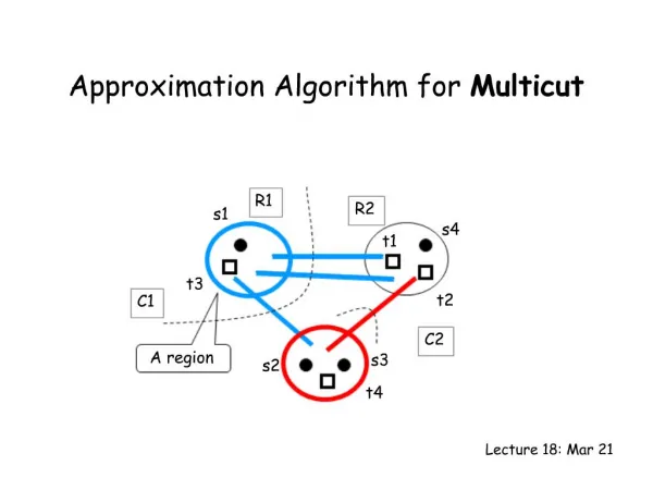
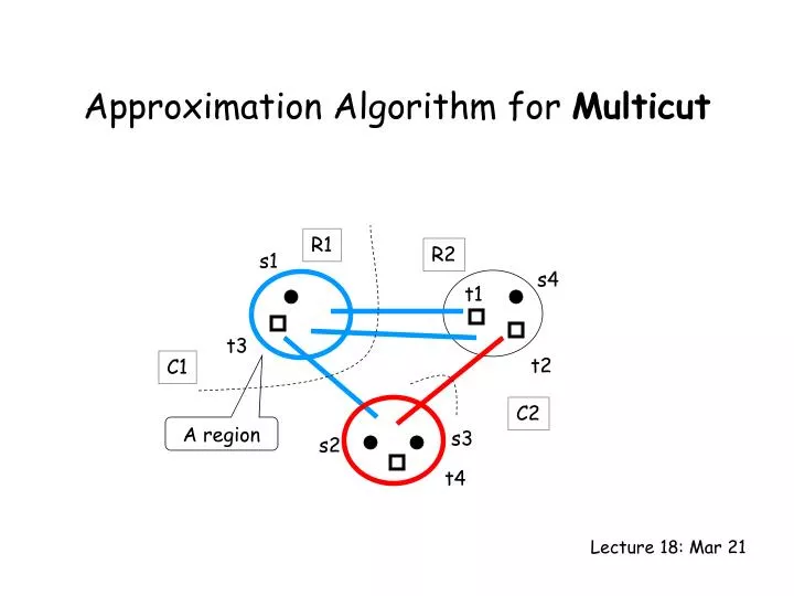
Approximation Algorithm for Multicut. R1. R2. s1. s4. t1. Lecture 18: Mar 21. t3. t2. C1. C2. A region. s3. s2. t4. Multiway Cut. Given a set of terminals S = {s1, s2, …, sk}, a multiway cut is a set of edges whose removal disconnects the terminals from each other.

E N D
Approximation Algorithm for Multicut R1 R2 s1 s4 t1 Lecture 18: Mar 21 t3 t2 C1 C2 A region s3 s2 t4
Multiway Cut Given a set of terminals S = {s1, s2, …, sk}, a multiway cut is a set of edges whose removal disconnects the terminals from each other. The multiway cut problem asks for the minimum weight multiway cut. s1 s2 s3 s4
Multiway Cut Algorithm • (Multiway cut 2-approximation algorithm) • For each i, compute a minimum weight isolating cut for s(i), say C(i). • Output the union of C(i). T2 s1 s2 T1 T3 T4 s3 s4
Multicut Given k source-sink pairs {(s1,t1), (s2,t2), ...,(sk,tk)}, a multicut is a set of edges whose removal disconnects each source-sink pair. The multicut problem asks for the minimum weight multicut. s1 s4 t1 t3 t2 s3 s2 t4
Bad Example Algorithm: take the union of minimum si-ti cut. t1 s1 1 1 s2 t2 1 1 2.0001 …….. 1 …….. 1 sk tk • OPT = 2.0001 • ALG = 2k
LinearProgram for each path p connecting a source-sink pair Intuitively, we would like to take edges with large d(e), but they may not form a multicut. How can we “round” this linear program?
Strategy s1 s4 0.3 t1 Let the edges in this multicut be C. t3 0.007 t2 0.2 0.01 s3 s2 t4 Given the fractional value of d(e), how can we compare a multicut with the optimal value of the LP? It would be good if d(e) ≥ 1/2 (or 1/k) for every edge in C. Then we would have a 2-approximation algorithm (or k-approximation algorithm). But this is not true.
Strategy s1 s4 0.3 t1 Let the edges in this multicut be C. t3 0.007 t2 0.2 0.01 s3 s2 t4 Given the fractional value of d(e), how can we compare a multicut with the optimal value of the LP? It would also be good if ∑c(e) ≤ k∑c(e)d(e) for edges in C. Then we would have a k-approximation algorithm. But this is also not true.
Strategy s1 s4 0.3 t1 Let the edges in this multicut be C. t3 0.007 t2 0.2 0.01 Observation: we haven’t considered the edges inside the components. s3 s2 t4 Analysis strategy: If we can prove that then we have a f(n)-approximation algorithm. We’ll use this strategy. How to find such a multicut C?
Algorithm R1 s1 s4 Goal: Find a cut with t1 t3 t2 C1 C2 A region s3 s2 t4 R2 • (Multicut approximation algorithm) • For each i, compute a s(i)-t(i) cut, say C(i). • Remove C(i) and its component R(i) (its region) from the graph • Output the union of C(i).
Requirements s1 s4 Goal: Find a cut with t1 t3 t2 A region s3 s2 What do we need for C(i)? t4 Cost requirement: Feasibility requirement: There is no source-sink pair in each R(i).
R1 R2 s1 s4 t1 t3 t2 C1 C2 A region s3 s2 t4 Cost Requirement Goal: Find a cut with Cost requirement: Cost requirement implies the Goal: It is important that every edge is counted at most once, and this is why we need to remove C(i) and R(i) from the graph.
LinearProgram Question: How to find the cut, i.e. R(i) and C(i), to satisfy the requirements? for each path p connecting a source-sink pair A useful interpretation is to think of d(e) as the length of e. So the linear program says that each source-sink pair is of distance at least 1.
Distance Key: think of d(e) as the length of e. Define the distance between two vertices as the length of their shortest path. Given a vertex v as the center, define S(r) to be the set of vertices of distance at most r from v. Idea: Set R(i) be to be S(r) with s1 as the center. R1 s1 Then, naturally, set C(i) to be the set of edges with one endpoint in R(i) and one endpoint outside R(i). C1
Feasibility Requirement Feasibility requirement: There is no source-sink pair in each R(i). This is because we’ll remove R(i) from the graph. The linear program says that each source-sink pair is of distance at least 1. Idea: Only choose S(r) with r ≤ ½. Radius ≤ ½ Since the distance between s(i) and t(i) is at least 1, they cannot be in the same R(j), and hence the feasibility requirement is satisfied. A region defined by a ball
Where are we? • (Multicut approximation algorithm) • For each i, compute a s(i)-t(i) cut, say C(i). • Remove C(i) and its component R(i) (its region) from the graph • Output the union of C(i). Use the idea of ball to find R(i) and C(i) The ball has to satisfy two requirements: Cost requirement: Feasibility requirement: There is no source-sink pair in each R(i). By choosing the radius at most ½
Finding Cheap Regions Ri Cost requirement: si Want: f(n) to be as small as possible. Ci Region growing: search from S(0) to S(1/2)! • Continuous process: think of dges as infinitely short. • set R(i) = S(r); initially r=0. • check if cost requirement is satisfied. • if not, increase r and repeat.
Exponential Increase Ri Cost requirement: si Ci If the cost requirement is not satisfied, we make the ball bigger. Note that the right hand side increases in this process, and so the left hand side also increases faster, and so on. In fact, the right hand side grows exponentially with the radius.
Logarithmic Factor Let , the optimal value of the LP. We only need to grow k regions, where k is the number of source-sink pairs. Set wt(S(0)) = F/k. In other words, we assign some additional weights to each source, but the total additional weight is at most F. Maximum weight a ball can get is F + F/k, from all the edges and the source. Set f(n) = 2ln(k+1).
Logarithmic Factor To summarize: By using the technique of region growing, we can find a cut (a ball with radius at most ½) that satisfies: Cost requirement: Feasibility requirement: There is no source-sink pair in each R(i). The cost requirement implies that it is an O(ln k)-approximation algorithm. The analysis is tight. The integrality gap of this LP is acutally Ω(ln k).
The Algorithm • (Multicut approximation algorithm) • Solve the linear program. • For each i, compute a s(i)-t(i) cut, say C(i). • Remove C(i) and its component R(i) (its region) from the graph • Output the union of C(i). • (Region growing algorithm) • Assign a weight F/k to s(i), and set S={s(i)}. • Add vertices to S in increasing order of their distances from s(i). • Stop at the first point when c(S), the total weight of the edges on the boundary, is at most 2ln(k+1)wt(S). • Set R(i):=S, and C(i) be the set of edges crossing R(i).
The Algorithm R1 s1 s4 t1 t3 t2 C1 C2 A region s3 s2 t4 R2
The Algorithm R1 s1 s4 t1 t3 t2 C1 C2 A region s3 s2 t4 • Important ideas: • Use linear program. • Compare the cost of the cut to the cost of the region. • Think of the variables as distances. • Growing the ball to find the region. R2 The idea of region growing can also be applied to other graph problems, most notably the feedback arc set problem, and also many applications.