Download
1 / 108
1.1k likes | 1.27k Views
A -Approximation Algorithm for Shortest Superstring. Sweedyk, Z. SIAM Journal on Computing, Vol. 29, No. 3, 1999, pp. 954-986. Speaker: Chuang-Chieh Lin Advisor: R. C. T. Lee National Chi-Nan University. Outline. Introduction Basic definitions String functions

E N D
A -Approximation Algorithm for Shortest Superstring Sweedyk, Z. SIAM Journal on Computing, Vol. 29, No. 3, 1999, pp. 954-986 Speaker: Chuang-Chieh Lin Advisor: R. C. T. Lee National Chi-Nan University
Outline • Introduction • Basic definitions • String functions • The approximation algorithm • The upper bound • The lower bound • Conclusion
Outline • Introduction • Basic definitions • String functions • The approximation algorithm • The upper bound • The lower bound • Conclusion
Introduction • Let S = {s1, s2, …, sn} be a set of strings. A superstring of S is a string containing each as a contiguous substring. • The shortest superstring problem is to find a minimum length superstring of the input set S. • This problem has important applications in computational biology and in data compression.
For example, S = { ab, bcd, de, abc }, then abcde is a superstring of length 5of S and abcabcde is a superstring of length 8of S.
Outline • Introduction • Basic definitions • String functions • The approximation algorithm • The upper bound • The lower bound • Conclusion
Basic definitions Let’s introduce some basic definitions.
Overlap • Let s and t be two strings. Let the suffix f of s and the prefix p of t are the same, then we call f or p the overlap of s with respect to t . • For example, s= cabab t = babcba bab is the overlap of s with respect to t.
OV (s, t) OV (s, t) is the set of overlaps of s with respect to t. For example, s= cabab, t = bababa OV (s, t) = {ε, b, bab }, OV (s, s) = {ε}, OV (t, t) = {ε, ba, baba }, OV (t, s) = {ε}.
ov(s, t), pref (s, t) and suff (s, t) • We use ov(s, t) to denote the longest string in OV(s, t); pref(s, t) and suff(s, t) denote the prefix of s and suffix of t corresponding to ov(s, t). • Furthermore, we use δS to denote pref(s, s) • For example, u1= cabab u1 = cabab u2 = bababa u2 = bababa u1 = cabab u2 = bababa So, pref (u1, u2) = ca, suff (u1, u2) = aba,
Distance/ overlap graph • Let S be a set of strings. The distance/ overlap graph GS is a complete diagraph with vertex set S; each edge of the graph is assigned a positive length as follows. • the edge e from s to t has length | e | = | pref (s, t) |.
For example, S = { u0, u1, u2}, where u0 = ababc, u1 = cabab, u2 = bababa . The following graph is GS . 1 5 5 4 u1 u0 u0 = ababc 6 u1 = cabab 3 2 5 u2 u1 = cabab u0 = ababc 2
The distance/ overlap multigraph gS • We define overlapov (e) = ov (s, t). • The distance/ overlap multigraph gS for S is constructed out of the distance/ overlap graph. Every and every an edge from s to t has length and overlap | v |.
For example,S = {u0, u1, u2} u0 = ababc, u1 = cabab, u2 = bababa 1, 4 5, 0 5, 0 4, 1 u1 u0 6, 0 3, 3 2, 3 5, 0 We use “m, n” to denote the “length and the overlap” of that edge. u2 2, 4
Why are the above graph useful? • Consider the Hamiltonian path u0-u1-u2. Its total overlap is 1 + 3 = 4. The corresponding superstring is ababcabababa (12) • Consider the Hamiltonian path u1-u2-u0. Its total overlap is 3 + 3 = 6. Its corresponding superstring is cababababc (10) (optimal solution).
Roughly speaking, we are interested in a cycle which covers all vertices with the largest sum of overlaps, or the smallest sum of lengths.
We have oversimplified the problem, because there may well be more than one cycle in the cycle cover. • In this case, we have to combine cycles.
Cycle cover • A cycle cover of GS is a set of simple cycles that cover all the vertices of the graph.
The following cycle c = (u0, u1, u2) is a cycle cover of GS 4, 1 u1 u0 3, 3 2, 3 u2 c where S = { u0, u1, u2 }, u0 = ababc, u1 = cabab, u2 = bababa
S = { u0, u1, u2 }, u0 = ababc, u1 = cabab, u2 = bababa • The following cycles also form a cycle cover of GS . 1, 4 4, 1 u1 u0 u2 2, 4
4, 1 • The following red and blue cycles also form a cycle cover. 5, 1 v1 4, 2 5, 0 5, 0 2, 3 6, 0 v0 5, 0 4, 0 v2 5, 0 5, 0 6, 0 5, 1 4, 0 3, 2 5, 0 4, 1 4, 0 3, 2 5, 0 v4 4, 0 v3 4, 1 4, 0 4, 1 3, 2
A minimum-length cycle cover CS* is a cycle cover of GS with minimum sum of lengths of edges. • The greedy algorithm can be used to construct CS*.
Since each cycle cover corresponds to several superstrings, the minimum cycle cover somehow corresponds to a rather shortsuperstring.
4, 1 • For example, Let S = {v1, v2, v3, v4, v5} v0 = aggtt, v1 = gttaag, v2 = taagc, v3 = gcata, v4 = tacc. Then gS is as follows: 5, 1 v1 4, 2 5, 0 5, 0 2, 3 6, 0 v0 5, 0 4, 0 v2 5, 0 5, 0 6, 0 5, 1 4, 0 3, 2 5, 0 4, 1 4, 0 3, 2 5, 0 v4 4, 0 v3 4, 1 4, 0 4, 1 3, 2
And we proceed the greedy algorithm to construct CS* : v0 = aggtt, v1 = gttaag, v2 = taagc, v3 = gcata, v4 = tacc 4, 1 5, 1 v1 4, 2 5, 0 5, 0 2, 3 6, 0 v0 4, 0 5, 0 v2 5, 0 5, 0 6, 0 5, 1 4, 0 3, 2 5, 0 4, 1 4, 0 3, 2 5, 0 v4 4, 0 v3 4, 1 4, 0 4, 1 3, 2
4, 1 5, 1 v1 4, 2 5, 0 5, 0 2, 3 6, 0 v0 4, 0 5, 0 v2 5, 0 5, 0 6, 0 5, 1 4, 0 3, 2 5, 0 4, 1 4, 0 3, 2 5, 0 v4 4, 0 v3 4, 1 4, 0 4, 1 3, 2
4, 1 5, 1 v1 4, 2 5, 0 5, 0 2, 3 6, 0 v0 4, 0 5, 0 v2 5, 0 5, 0 6, 0 5, 1 4, 0 3, 2 5, 0 4, 1 4, 0 3, 2 5, 0 v4 4, 0 v3 4, 1 4, 0 4, 1 3, 2
4, 1 5, 1 v1 4, 2 5, 0 5, 0 2, 3 6, 0 v0 4, 0 5, 0 v2 5, 0 5, 0 6, 0 5, 1 4, 0 3, 2 5, 0 4, 1 4, 0 3, 2 5, 0 v4 4, 0 v3 4, 1 4, 0 4, 1 3, 2
4, 1 5, 1 v1 4, 2 5, 0 5, 0 2, 3 6, 0 v0 4, 0 5, 0 v2 5, 0 5, 0 6, 0 5, 1 4, 0 3, 2 5, 0 4, 1 4, 0 3, 2 5, 0 v4 4, 0 v3 4, 1 4, 0 4, 1 3, 2
4, 1 5, 1 v1 4, 2 5, 0 5, 0 2, 3 6, 0 v0 4, 0 5, 0 v2 5, 0 5, 0 6, 0 5, 1 4, 0 3, 2 5, 0 4, 1 4, 0 3, 2 5, 0 v4 4, 0 v3 4, 1 4, 0 4, 1 3, 2
Now, the following graph is CS* v0 = aggtt, v1 = gttaag, v2 = taagc, v3 = gcata, v4 = tacc v1 4, 2 2, 3 c1 v0 v2 3, 2 c2 3, 2 v4 c3 v3 4, 0
v0 = aggtt, v1 = gttaag, v2 = taagc, v3 = gcata, v4 = tacc. • The superstrings corresponding to the cycles of this cycle cover are as follows v0 - v1: aggttaag v2 - v3: taagcata v4: tacc The superstring: aggttaagtaagcatacc can be obtained by concatenating the three cycles.
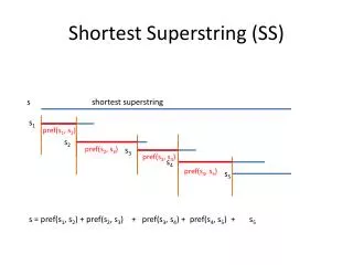
Open • Let c = (s0, s1,…, sj-1, s0) be a cycle of GS. For any l , the string , where the indices are taken modulo j, is called an open of c.
A cycle c may have many opens. We can regard opens as local superstrings.
For example, 1, 4 u0 = ababc u1 = cabab u2 = bababa c1 = (u2, u2) c2 = (u0, u1, u0) 4, 1 u1 u0 c2 u2 4, 2 c1 Let x1 = bababa, x21 = ababcabab, x22 = cababc x1 is an open of c1. x21 and x22 are opens of c2.
For any cycle c, an open is a Hamiltonian path of this cycle.
For example, 1, 4 u0 = ababc u1 = cabab u2 = bababa c1 = (u2, u2) c2 = (u0, u1, u0) OP(c1) = { bababa } OP(c2) = { ababcabab, cababc } 4, 1 u1 u0 c2 u2 4, 2 c1
The vertices are called, respectively, xfirst and xlastand the edge <xlast,xfirst > is called the opening edge of x. An opening edge of x is an edge whose removal creates the open x. For example, <u2, u2> is the opening edge of x1 <u1, u0> is the opening edge of x21
Lemma 2.12 • Let c be a cycle. We denote sop(c) to be the shortest open of c. If the minimum length cycle cover CS* consists of a single cycle c, sop(c) is a shortest superstring of S.
For example, Cycle cover c2is a minimum length cycle cover and c2 consists of just one cycle. OP(c2) = { ababcabab, cababc }. So sop (c2) = cababc is a shortest superstring of u0 = ababc and u1 = cabab. 1, 4 4, 1 u1 u0 c2
Outline • Introduction • Basic definitions • String functions • The approximation algorithm • The upper bound • The lower bound • Conclusion
String functions and lemmas • At first, we should know the meaning of the expansion of a cycle or an edge.
Expansion • e = < s, t, k > and are versions of each other and if , we say that e is an expansion of • For example, s = bbcabba, t = abbabab bbcabba bbcabba abbabab abbabab • Let e = < s, t, 1>, . Therefore, e is an expansion of .
1-expansion • is an expansion of c if every edge of is an expansion of an edge in c. • An edge < s, t, k > is tight if k = |ov (s, t)| and loose otherwise. • We call a cycle of gS a 1-expansion of if is an expansion of c and it has only one loose edge.
When we refer to a 1-expansion of cx for , we mean that the only possible loose edge is <xlast, xfirst>. • For example, • is a 1-expansion of . 1, 4 3, 2 4, 1 4, 1 u1 u1 u0 u0 u1 = cabab u1 = cabab u0 = ababc u0 = ababc
Let’s take a look at an example here with 3 strings where an expansion of the superstring of two strings should be expanded so that the final superstring covering the three strings is even shorter.
y1 = abcd, y2 = cdba, y3 = cdcdbaba Case 1: without expansion: y1= abcd y2 = cdba y12 = abcdba y12 = abcdba y123 = cdcdbababcdba y3 = cdcdbaba Case 2: with expansion: y1= abcd y2 = cdba y12 = abcdcdba y12 = abcdcdba y123 = cdcdbaba y3 = cdcdbaba
The above example shows we have to consider some string functions to improve our solutions.