Download
1 / 151
1.61k likes | 2.86k Views
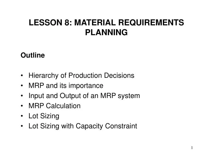
LESSON 8: MATERIAL REQUIREMENTS PLANNING. Outline Hierarchy of Production Decisions MRP and its importance Input and Output of an MRP system MRP Calculation Lot Sizing Lot Sizing with Capacity Constraint. Hierarchy of Production Decisions.

E N D
LESSON 8: MATERIAL REQUIREMENTS PLANNING Outline • Hierarchy of Production Decisions • MRP and its importance • Input and Output of an MRP system • MRP Calculation • Lot Sizing • Lot Sizing with Capacity Constraint
Hierarchy of Production Decisions • The next slide presents a schematic view of the aggregate production planning function and its place in the hierarchy of the production planning decisions. • Forecasting: First, a firm must forecast demand for aggregate sales over the planning horizon. • Aggregate planning: The forecasts provide inputs for determining aggregate production and workforce levels over the planning horizon. • Master production schedule (MPS): Recall, that the aggregate production plan does not consider any “real” product but a “fictitious” aggregate product. The MPS translates the aggregate plan output in terms of specific production goals by product and time period. For example,
Hierarchy of Production Decisions suppose that a firm produces three types of chairs: ladder-back chair, kitchen chair and desk chair. The aggregate production considers a fictitious aggregate unit of chair and find that the firm should produce 550 units of chairs in April. The MPS then translates this output in terms of three product types and four work-weeks in April. The MPS suggests that the firm produce 200 units of desk chairs in Week 1, 150 units of ladder-back chair in Week 2, and 200 units of kitchen chairs in Week 3. • Material Requirements Planning (MRP): A product is manufactured from some components or subassemblies. For example a chair may require two back legs, two front legs, 4 leg supports, etc. While forecasting, aggregate plan
Hierarchy of Production DecisionsMaster Production Schedule April May 1 2 3 4 5 6 7 8 Ladder-back chair 150 150 200 Kitchen chair 120 120 Desk chair 200 200 200 Aggregate production plan 790 550 for chair family
Hierarchy of Production Decisions and MPS consider the volume of finished products, MRP plans for the components, and subassemblies. A firm may obtain the components by in-house production or purchasing. MRP prepares a plan of in-house production or purchasing requirements of components and subassemblies. • Scheduling: Scheduling allocates resource over times in order to produce the products. The resources include workers, machines and tools. • Vehicle Routing: After the products are produced, the firm may deliver the products to some other manufacturers, or warehouses. The vehicle routing allocates vehicles and prepares a route for each vehicle.
Hierarchy of Production DecisionsMaterials Requirement Planning Back slats Seat cushion Leg supports Seat-frame boards Back legs Front legs
Material Requirements Planning • The demands for the finished goods are obtained from forecasting. These demands are called independent demand. • The demands for the components or subassemblies depend on those for the finished goods. These demands are called dependent demand. • Material Requirements Planning (MRP) is used for dependent demand and for both assembly and manufacturing • If the finished product is composed of many components, MRP can be used to optimize the inventory costs.
Importance of an MRP System • Next two slides explain the importance of an MRP system. The first one shows inventory levels when an MRP system is not used. The next one shows the same when an MRP system is used. • The chart at the top shows inventory levels of the finished goods and the chart on the bottom shows the same of the components. • If the production is stopped (like it is at the beginning of the chart), the finished goods inventory level decreases because of sales. However, the component inventory level remains unchanged. When the production resumes, the finished goods inventory level increases, but the component inventory level decreases.
Importance of an MRP System Inventory without an MRP System
Importance of an MRP System Inventory with an MRP System
Importance of an MRP System • Without an MRP system: • Component is ordered at time A, when the inventory level of the component hits reorder point, R • So, the component is received at time B. • However, the component is actually needed at time C, not B. So, the inventory holding cost incurred between time B and C is a wastage. • With an MRP system: • We shall see in this lesson that given the production schedule of the finished goods and some other information (see the next slide), it is possible to predict the exact time, C when the component will be required. Order is placed carefully so that it is received at time C.
MRP Input and Output • MRP Inputs: • Master Production Schedule (MPS): The MPS of the finished product provides information on the net requirement of the finished product over time. • Bill of Materials: For each component, the bill of materials provides information on the number of units required, source of the component (purchase/ manufacture), etc. There are two forms of the bill of materials: • Product Structure Tree: The finished product is shown at the top, at level 0. The components assembled to produce the finished product is shown at level 1 or below. The sub-components used to produce the components at level 1 is
MRP Input and Output Master Production Schedule Orders Forecasts Bill of Materials file MRP computer program Inventory file Reports To Production To Purchasing
MRP Input and Output shown at level 2 or below, and so on. The number in the parentheses shows the requirement of the item. For example, “G(4)” implies that 4 units of G is required to produce 1 unit of B. The levels are important. The net requirements of the components are computed from the low levels to high. First, the net requirements of the components at level 1 is computed, then level 2, and so on.
MRP Input and Output • Bill of Materials: For each item, the name, number, source, and lead time of every component required is shown on the bill of materials in a tabular form. • Inventory file: For each item, the number of units on hand is obtained from the inventory file. • MRP Output: • Every required item is either produced or purchased. So, the report is sent to production or purchasing.
Bill of Materials: Product Structure Tree Level 0 Level 1 Level 2 Level 3
On Hand Inventory and Lead time Component Units in Lead Inventory time (weeks) Seat Subassembly 25 2 Seat frame 50 3 Seat frame boards 75 1
MRP Calculation • Now, the MRP calculation will be demonstrated with an example. • Suppose that 150 units of ladder-back chair is required. • The previous slide shows a product structure tree with seat subassembly, seat frames, and seat frame boards. For each of the above components, the previous slide also shows the number of units on hand. • The net requirement is computed from top to bottom. Since 150 units of ladder-back chair is required, and since 1 unit of seat subassembly is required for each unit of ladder-back chair, the gross requirement of seat-subassembly is 1501 =150 units. Since there are 25 units of seat-subassembly in the inventory, the net requirement of the seat-subassembly is 150-25 = 125
MRP Calculation units. Since 1 unit of seat frames is required for each unit of seat subassembly, the gross requirement of the seat frames is 1251 = 125 units. (Note that although it follows from the product structure tree that 1 unit of seat frames is required for each unit of ladder-back chair, the gross requirement of seat frames is not 150 units because each of the 25 units of seat-subassembly also contains 1 unit of seat frames.) Since there are 50 units of seat frames in the inventory, the net requirement of the seat frames is 125-50 = 75 units. The detail computation is shown in the next two slides. • A similar logic is used to compute the time of order placement.
MRP Calculation Assume that 150 units of ladder-back chairs are to be produced at the end of week 15
MRP Calculation: Time of Order Placement Assume that 150 units of ladder-back chairs are to be produced at the end of week 15 and that there is a one-week lead time for ladder-back chair assembly
MRP Calculation: Some Definitions • Scheduled Receipts: • Items ordered prior to the current planning period and/or • Items returned from the customer • Lot-for-lot (L4L) • Order quantity equals the net requirement • Sometimes, lot-for-lot policy cannot be used. There may be restrictions on minimum order quantity or order quantity may be required to multiples of 50, 100 etc.
MRP Calculation Example 1: Each unit of A is composed of one unit of B, two units of C, and one unit of D. C is composed of two units of D and three units of E. Items A, C, D, and E have on-hand inventories of 20, 10, 20, and 10 units, respectively. Item B has a scheduled receipt of 10 units in period 1, and C has a scheduled receipt of 50 units in Period 1. Lot-for-lot (L4L) is used for Items A and B. Item C requires a minimum lot size of 50 units. D and E are required to be purchased in multiples of 100 and 50, respectively. Lead times are one period for Items A, B, and C, and two periods for Items D and E. The gross requirements for A are 30 in Period 2, 30 in Period 5, and 40 in Period 8. Find the planned order releases for all items.
MRP Calculation Level 0 Level 1 Level 2
MRP Calculation 30 30 40 20 1 WK L4L All the information above are given.
MRP Calculation 30 30 40 20 20 1 WK -- L4L 20 units are just transferred from Period 1 to 2.
MRP Calculation 30 30 40 20 20 1 WK 10 -- 10 L4L 10 10 The net requirement of 30-20=10 units must be ordered in week 1.
MRP Calculation 30 30 40 20 20 0 0 0 1 WK 10 -- 10 L4L 10 10 On hand in week 3 is (20+10)-30=0 unit.
MRP Calculation 30 30 40 20 20 0 0 0 1 WK 30 10 -- 30 10 L4L 30 10 10 30 The net requirement of 30-0=30 units must be ordered in week 4.
MRP Calculation 30 30 40 20 20 0 0 0 0 0 0 1 WK 30 40 10 -- 30 40 10 L4L 30 40 10 10 30 40 The net requirement of 40-0=30 units must be ordered in week 7.
MRP Calculation 30 30 40 20 20 0 0 0 0 0 0 0 0 1 WK 30 40 10 -- 30 40 10 L4L 30 40 10 10 30 40 The net requirement of 40-0=30 units must be ordered in week 7.
MRP Calculation Exercise
MRP Calculation Exercise
MRP Calculation Exercise
MRP Calculation Exercise
READING AND EXERCISES Lesson 8 Reading: Section 7.1 pp. 355-364 (4th Ed.), pp. 346-358 (5th Ed.) Exercise: 4 and 9 pp. 364-366 (4th Ed.), pp. 356-358 (5th Ed.)
LESSON 9: MATERIAL REQUIREMENTS PLANNING: LOT SIZING Outline • Lot Sizing • Lot Sizing Methods • Lot-for-Lot (L4L) • EOQ • Silver-Meal Heuristic • Least Unit Cost (LUC) • Part Period Balancing
Lot-Sizing • In Lesson 21 • We employ lot for lot ordering policy and order production as much as it is needed. • Exception are only the cases in which there are constraints on the order quantity. • For example, in one case we assume that at least 50 units must be ordered. In another case we assume that the order quantity must be a multiple of 50. • The motivation behind using lot for lot policy is minimizing inventory. If we order as much as it is needed, there will be no ending inventory at all!
Lot-Sizing • However, lot for lot policy requires that an order be placed each period. So, the number of orders and ordering cost are maximum. • So, if the ordering cost is significant, one may naturally try to combine some lots into one in order to reduce the ordering cost. But then, inventory holding cost increases. • Therefore, a question is what is the optimal size of the lot? How many periods will be covered by the first order, the second order, and so on until all the periods in the planning horizon are covered. This is the question of lot sizing. The next slide contains the statement of the lot sizing problem.
Lot-Sizing • The lot sizing problem is as follows: Given net requirements of an item over the next T periods, T >0, find order quantities that minimize the total holding and ordering costs over T periods. • Note that this is a case of deterministic demand. However, the methods learnt in Lessons 11-15 are not appropriate because • the demand is not necessarily the same over all periods and • the inventory holding cost is only charged on ending inventory of each period
Lot-Sizing • Although we consider a deterministic model, keep in mind that in reality the demand is uncertain and subject to change. • It has been observed that an optimal solution to the deterministic model may actually yield higher cost because of the changes in the demand. Some heuristic methods give lower cost in the long run. • If the demand and/or costs change, the optimal solution may change significantly causing some managerial problems. The heuristic methods may not require such changes in the production plan. • The heuristic methods require fewer computation steps and are easier to understand. • In this lesson we shall discuss some heuristic methods. The optimization method is discussed in the text, Appendix 7-A, pp 406-410 (not included in the course).
Lot-Sizing • Some heuristic methods: • Lot-for-Lot (L4L): • Order as much as it is needed. • L4Lminimizes inventory holding cost, but maximizes ordering cost. • EOQ: • Every time it is required to place an order, lot size equals EOQ. • EOQ method may choose an order size that covers partial demand of a period. For example, suppose that EOQ is 15 units. If the demand is 12 units in period 1 and 10 units in period 2, then a lot size of 15 units covers all of period 1 and only (15-12)=3 units of period 2. So, one does not save the ordering cost of period 2, but carries some 3 units in
Lot-Sizing • Some heuristic methods: the inventory when that 3 units are required in period 2. This is not a good idea because if an order size of 12 units is chosen, one saves on the holding cost without increasing the ordering cost! • So, what’s the mistake? Generally, if the order quantity covers a period partially, one can save on the holding cost without increasing the ordering cost. The next three methods, Silver-Meal heuristic, least unit cost and part period balancing avoid order quantities that cover a period partially. These methods always choose an order quantity that covers some K periods, K >0. • Be careful when you compute EOQ. Express both holding cost and demand over the same period. If the holding cost is annual, use annual demand. If the holding cost is weekly, use weekly demand.
Lot-Sizing • Some heuristic methods: • Silver-Meal Heuristic • As it is discussed in the previous slide, Silver-Meal heuristic chooses a lot size that equals the demand of some K periods in future, where K>0. • If K =1, the lot size equals the demand of the next period. • If K =2, the lot size equals the demand of the next 2 periods. • If K =3, the lot size equals the demand of the next 3 periods, and so on. • The average holding and ordering cost per period is computed for each K=1, 2, 3, etc. starting from K=1 and increasing K by 1 until the average cost per period starts increasing. The best K is the last one up to which the average cost per period decreases.
Lot-Sizing • Some heuristic methods: • Least Unit Cost (LUC) • As it is discussed before, least unit cost heuristic chooses a lot size that equals the demand of some K periods in future, where K>0. • The average holding and ordering cost per unit is computed for each K=1, 2, 3, etc. starting from K=1 and increasing K by 1 until the average cost per unit starts increasing. The best K is the last one up to which the average cost per unit decreases. • Observe how similar is Silver-Meal heuristic and least unit cost heuristic. The only difference is that Silver-Meal heuristic chooses K on the basis of average cost per period and least unit cost on average cost per unit.
Lot-Sizing • Some heuristic methods: • Part Period Balancing • As it is discussed before, part period balancing heuristic chooses a lot size that equals the demand of some K periods in future, where K>0. • Holding and ordering costs are computed for each K=1, 2, 3, etc. starting from K=1 and increasing K by 1 until the holding cost exceeds the ordering cost. The best K is the one that minimizes the (absolute) difference between the holding and ordering costs. • Note the similarity of this method with the Silver-Meal heuristic and least unit cost heuristic. Part period balancing heuristic chooses K on the basis of the (absolute) difference between the holding and ordering costs.