Download
1 / 39
390 likes | 396 Views
This article explores the object-oriented modeling of heat and humidity budgets in Biosphere 2, an environmental research facility, using bond graphs. It discusses the construction of Biosphere 2, its biomes, climate control systems, and the conceptual modeling of temperature and humidity factors. The Dymola model and equations for evaporation, condensation, and atmospheric phenomena are also presented.

E N D
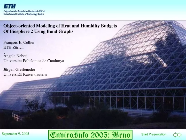
François E. Cellier ETH Zürich Àngela Nebot Universitat Politècnica de Catalunya Jürgen Greifeneder Universität Kaiserslautern Object-oriented Modeling of Heat and Humidity Budgets Of Biosphere 2 Using Bond Graphs
Biosphere 2 is an environmental research facility, located in the desert of Southern Arizona, that allows performing experiments in a materially closed ecological system under controlled experimental conditions. What is Biosphere 2 • Biosphere 2 was built around 1990 with private funding and has functioned for almost 15 years already for various ecological experiments.
In Biosphere 1 (the Earth ecosystem), it is difficult to perform experiments, because of limited access to control variables. Why Biosphere 2 • In Biosphere 1, it is easy to observe phenomena and report them, but it is difficult to interpret these observations in an objective fashion. • In Biosphere 1, we are able to correlate data, but correlations per se do not establish cause and effect relationships.
Biosphere 2 was built as a frame construction from a mesh of metal bars. The metal bars are filled with glass panels that are well insulated. During its closed operation, Biosphere 2 was slightly over-pressurized to prevent outside air from entering the structure. The air loss per unit volume was about 10% of that of the space shuttle! Biosphere 2: Construction
The pyramidal structure hosts the jungle biome. The less tall structure to the left contains the pond, the marshes, the savannah, and at the lowest level, the desert. Though not visible on the photograph, there exists yet one more biome: the agricultural biome. Biosphere 2: Construction II
The two “lungs” are responsible for pressure equilibration within Biosphere 2. Each lung contains a heavy concrete ceiling that is flexibly suspended and insulated with a rubber membrane. If the temperature within Biosphere 2 rises, the inside pressure rises as well. Biosphere 2: Construction III Consequently, the ceiling rises until the inside and outside pressure values are again identical. The weight of the ceiling is responsible for providing a slight over-pressurization of Biosphere 2.
The (salt water) pond of Biosphere 2 hosts a fairly complex maritime ecosystem. Visible behind the pond are the marsh lands planted with mangroves. Artificial waves are being generated to keep the mangroves healthy. Above the cliffs to the right, there is the high savannah. Biosphere 2: Biomes
This is the savannah. Each biome uses its own soil composition sometimes imported, such as in the case of the rain forest. Biosphere 2 has 1800 sensors to monitor the behavior of the system. Measurement values are recorded on average once every 15 Minutes. Biosphere 2: Biomes II
The agricultural biome can be subdivided into three separate units. The second lung is on the left in the background. Biosphere 2: Biomes III
The Biosphere 2 library is located at the top level of a high tower with a spiral staircase. Living in Biosphere 2 The view from the library windows over the Sonora desert is spectacular.
From the commando unit, it is possible to control the climate of each biome individually. For example, it is possible to program rain over the savannah to take place at 3 p.m. during 10 minutes. The Rain Maker
The climate control unit (located below ground) is highly impressive. Biosphere 2 is one of the most complex engineering systems ever built by mankind. Climate Control
Beside from the temperature, also the humidity needs to be controlled. To this end, the air must be constantly dehumidified. The extracted water flows to the lowest point of the structure, located in one of the two lungs, where the water is being collected in a small lake; from there, it is pumped back up to where it is needed. Climate Control II
Temperature Humidity Condensation Evaporation The Bond-Graph Model For evaporation, energy is needed. This energy is taken from the thermal domain. In the process, so-called latent heat is being generated. In the process of condensation, the latent heat is converted back to sensible heat. The effects of evaporation and condensation cannot be neglected in the modeling of Biosphere 2.
The overall Dymola model is shown to the left. At least, the picture shown is the top-level icon window of the model. The Dymola Model
Night Sky Temperature Temperature of Cover Ambient Temperature Air Temperature Vegetation Temperature Air Humidity Soil Temperature Water Temperature The Dymola Model II
Night Sky Radiation Solar Convection Solar Radiation Convection Evaporation and Condensation The Dymola Model III
e2 e1 Gth = G / T T T = e1+ e2 Convection Rth = R · T
e1 Gth = G · T 2 e1 T = e1 Radiation Rth = R / T 2
Programmed as equations Teten’s law } Sensible heat in = latent heat out Evaporation of the Pond
Programmed as equations If the temperature falls below the dew point, fog is created. Condensation in the Atmosphere
The ambient temperature is computed here by interpolation from a huge temperature data file. Data were available for the location of Tucson only. Correction factors were used to estimate the effects of the higher altitude of Oracle. Ambient Temperature
Absorption, Reflection, Transmission Since the glass panels are pointing in all directions, it would be too hard to compute the physics of absorption, reflection, and transmission accurately, as we did in the last example. Instead, we simply divide the incoming radiation proportionally.
Distribution of Absorbed Radiation The absorbed radiation is railroaded to the different recipients within the overall Biosphere II structure.
Not bad! The Dymola Biosphere Package We are now ready to compile and simulate the Biosphere model. (The compilation is still fairly slow, because Dymola isn’t geared yet to deal with such large measurement data files.)
The program works with weather data that record temperature, radiation, humidity, wind velocity, and cloud cover for an entire year. Without climate control, the inside temperature follows essentially outside temperature patterns. There is some additional heat accumulation inside the structure because of reduced convection and higher humidity values. Simulation Results I
Since water has a larger heat capacity than air, the daily variations in the pond temperature are smaller than in the air temperature. However, the overall (long-term) temperature patterns still follow those of the ambient temperature. Simulation Results II
The humidity is much higher during the summer months, since the saturation pressure is higher at higher temperature. Consequently, there is less condensation (fog) during the summer months. Indeed, it can be frequently observed that during spring or fall evening hours, after sun set, fog starts to build over the high savannah, which then migrates to the rain forest, which eventually gets totally fogged in. Simulation Results III
Daily temperature variations in the summer months. The air temperature inside Biosphere 2 would vary by approximately 10oC over the duration of one day, if there were no climate control. Simulation Results IV
Temperature variations during the winter months. Also in the winter, daily temperature variations are approximately 10oC. The humidity variations follow the temperature variations almost exactly. This observation shall be explained at once. Simulation Results V
The relative humidity is computed as the quotient of the true humidity and the humidity at saturation pressure. The atmosphere is almost always saturated. Only in the late morning hours, when the temperature rises rapidly, will the fog dissolve so that the sun may shine quickly. However, the relative humidity never decreases to a value below 94%. Only the climate control (not included in this model) makes life inside Biosphere II possible. Simulation Results VI
In a closed system, such as Biosphere 2, evaporation necessarily leads to an increase in humidity. However, the humid air has no mechanism to ever dry up again except by means of cooling. Consequently, the system operates almost entirely in the vicinity of 100% relative humidity. The climate control is accounting for this. The air extracted from the dome is first cooled down to let the water fall out, and only thereafter, it is reheated to the desired temperature value. However, the climate control was not simulated here. Modeling of the climate control of Biosphere 2 is still in the works. Simulation Results VII
Brück, D., H. Elmqvist, H. Olsson, and S.E. Mattsson (2002), “Dymola for Multi-Engineering Modeling and Simulation,” Proc. 2nd International Modelica Conference, pp. 55:1-8. Cellier, F.E. (1991), Continuous System Modeling, Springer-Verlag, New York. Cellier, F.E. and J. Greifeneder (2003), “Object-oriented Modeling of Convective Flows Using the Dymola Thermo-Bond-Graph Library,” Proc. ICBGM’03, 6th Intl. Conference on Bond Graph Modeling and Simulation, Orlando, Florida, pp. 198-204. References I
Cellier, F.E. and R.T. McBride (2003), “Object-oriented Modeling of Complex Physical Systems Using the Dymola bond-graph library,” Proc. ICBGM’03, Intl. Conference on Bond Graph Modeling and Simulation, Orlando, Florida, pp.157-162. Cellier, F.E. and A. Nebot (2005), “The Modelica Bond Graph Library,” Proc. 4th Modelica Conference, Hamburg, Germany, Vol. 1, pp. 57-65. Greifeneder, J. (2001), Modellierung thermodynamischer Phänomene mittels Bondgraphen, MS Thesis, Institut für Systemdynamik und Regelungstechnik, Universität Stuttgart, Germany. References II
Greifeneder, J. and F.E. Cellier (2001), “Modeling Convective Flows Using Bond Graphs,” Proc. ICBGM’01, 5th Intl. Conference on Bond Graph Modeling and Simulation, Phoenix, Arizona, pp. 276-284. Greifeneder, J. and F.E. Cellier (2001), “Modeling Multi-phase Systems Using Bond Graphs,” Proc. ICBGM’01, 5th Intl. Conference on Bond Graph Modeling and Simulation, Phoenix, Arizona, pp. 285-291. Greifeneder, J. and F.E. Cellier (2001), “Modeling Multi-element Systems Using Bond Graphs,” Proc. ESS’01, 13th European Simulation Symposium, Marseille, France, pp. 758-766. References III
Nebot, A., F.E. Cellier, and F. Mugica (1999), “Simulation of Heat and Humidity Budgets of Biosphere 2 Without Air Conditioning,” Ecological Engineering, 13, pp. 333-356. Cellier, F.E. (2005), The Dymola Bond Graph Library, Version 1.1. Cellier, F.E. (1997), Tucson Weather Data for Matlab. References IV