Download
1 / 24
240 likes | 326 Views
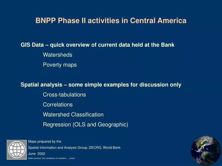
BNPP Phase II activities in Central America GIS Data – quick overview of current data held at the Bank Watersheds Poverty maps Spatial analysis – some simple examples for discussion only Cross-tabulations Correlations Watershed Classification Regression (OLS and Geographic).

E N D
BNPP Phase II activities in Central America GIS Data – quick overview of current data held at the Bank Watersheds Poverty maps Spatial analysis – some simple examples for discussion only Cross-tabulations Correlations Watershed Classification Regression (OLS and Geographic) Maps prepared by the Spatial Information and Analysis Group, DECRG, World Bank June 2002 Data sources, too numerous to mention…..sorry!
Population Density 1000+ administrative units, 35,000 per unit High Low
Elevation and derived products 100m resolution
Example: Terrain Typology 500m resolution Plains Lowlands Plateaus Mountains
1:250,000 Land Cover 100m resolution Forest Agriculture Urban Savanna 50% of forested land is in hillsides/mountainous areas
Other data sets Climate - 1km monthly rainfall and temperature data (2000) Fire - fire spots (1996-2000) and burn-scars (2000) Accessibility - to major cities, ports Protected areas Transport networks Rivers, lakes
Poverty maps: Guatemala Extreme Poverty Rate Extreme Poverty Headcount 100 80 60 40 20 0 High Low
Poverty maps: Nicaragua Extreme Rural Poverty Rate Extreme Rural Poverty Headcount 100 80 60 40 20 0 High Low
Watersheds: how many are there? Rio Paz
First level Second level Third level The best available population data is second level admin for all countries, with around 1,000 units and 35,000 people per unit. If we want to use these socio-economic data with watershed units, then we need around 1000 watersheds, of around 500km2 each. Other watershed analyses with no socio-economic data could use any size watershed, depending on the questions being asked.
Watersheds How to derive watersheds from Terrain and River data? What descriptive and useful characteristics can we generate? How many watersheds (scale/size issue)?
Example regression in Guatemalan Watersheds LHS = % of population in extreme poverty RHS = Watershed Shape Factor Road & Lane Density % Forest % Agriculture Elevation % Urban Forest/ Agriculture Interface Length R2 = 0.36 Parameter Estimate Std Err T --------- ------------ ------------ ------------ Intercept -0.033294 0.069684 -0.477786 Watershed Shape 0.027051 0.016371 1.652375 Road Density -0.047331 0.088072 -0.537422 Lane Density 0.189764 0.056036 3.386457 For/Agri Interface -0.029461 5.097628 -0.005779 Elevation 0.000104 0.000018 5.688500 % Agriculture 0.096577 0.065151 1.482350 % Forest 0.241825 0.070563 3.427060 % Urban -0.697173 0.507178 -1.374611
Geographic regression in Guatemalan Watersheds • For each watershed in turn (312 in this case) • Generate a list of the 99 nearest neighbours • Run regression on these 100 watersheds using a spatial weighting scheme, watersheds closer to the middle get a higher weighting • Assign regression results to the central watershed • Repeat for all watersheds • Map results, R2, beta coefficients, etc.
Geographic regression in Guatemalan Watersheds • Generate a regression for each watershed using its nearest 99 neighbours. • So for each watershed we have • A R2 value • A set of beta coefficients • A set of standard errors • etc… • Now it is possible to map the Beta coefficients and determine • If they vary significantly over space • If they flip from +ve to –ve influence in the regression R2 = 0.76 0 .2 .4 .6 .8 1.0
Geographic regression in Guatemalan Watersheds Global -0.0332 0.0270 -0.0473 0.1897 -0.0294 0.0001 0.0965 0.2418 -0.6971 5 number summaries for the variation in each parameter across space Label Minimum Lwr Quartile Median Upr Quartile Maximum Intrcept -0.838 -0.001 0.158 0.230 0.572 shape -0.055 0.008 0.016 0.034 0.140 Roads -0.510 -0.181 0.043 0.173 0.656 Lanes -0.502 0.002 0.123 0.232 0.561 Interfac -62.843 -9.260 2.199 15.831 65.038 m_ele -0.000 -0.000 0.000 0.000 0.000 Agricult -0.499 -0.073 0.023 0.129 0.508 Forest -0.627 -0.017 0.107 0.257 0.979 Urban -14.574 -4.359 -1.350 -0.104 5.180 Every coefficient varies from +ve to –ve influence over the region. -> Variations in relationships and processes(?) over space 4 of the coefficients vary significantly over space (Monte Carlo simulation)
Geographic regression in Guatemalan Watersheds % agriculture Agriculture Beta coefficient High Low High Low
Geographic regression in Guatemalan Watersheds If we classify each watershed based on its 9 beta coefficients…. Distinct spatial structure in the relationships between the coefficients.
Plenty of high resolution data for the region • Opportunity to explore spatial patterns / trends in • poverty / environment data • Opportunity to explore scale effects in those patterns • Need to relate this to the Phase II TORs