Download
1 / 28
290 likes | 431 Views
Spatial Alignment. Spring 2009. Ben-Gurion University of the Negev. Instructor. Dr. H. B Mitchell email: hmitchell@elta.co.il. Sensor Fusion Spring 2009. Spatial Alignment. Process of geometrically aligning images of the same scene acquired

E N D
Spatial Alignment Spring 2009 Ben-Gurion University of the Negev
Instructor • Dr. H. B Mitchell email: hmitchell@elta.co.il Sensor Fusion Spring 2009
Spatial Alignment • Process of geometrically aligning images of the same scene acquired • At different times (multi-temporal fusion) • With different sensors (multi-modal fusion) • From different viewpoints (multi-view fusion) Sensor Fusion Spring 2009
Example Sensor Fusion Spring 2009
Spatial Alignment Algorithms • Classify them by the nature of the images to register • Monomodal registration • Multimodal registration Sensor Fusion Spring 2009
Spatial Alignment • A: reference image • B: floating image • Spatial alignment finds transformation T which maps each pixel (x,y) in B into a location in A: B A (x,y) Sensor Fusion Spring 2009
Transformations • Some common transformations: Local Global transformations Sensor Fusion Spring 2009
Global Transformations • Translation • Similarity • Affine • Perspective • Polynomial Sensor Fusion Spring 2009
Spatial Alignment • The location does not correspond to a pixel location in A. • In order to convert the gray-level into a digital image which is defined at the same pixel locations as A we require an interpolation/resampling • Symbolically write it as Sensor Fusion Spring 2009
Spatial Alignment • Spatial alignment of B to A gives us • But we require • This is found by going in the reverse direction, i.e. from A to B A to B B to A Sensor Fusion Spring 2009
Spatial Alignment. Nearest Neighbor • Simplest resample/interpolation algorithm is nearest neighbor. • We have • Then find if is nearest pixel coordinates to then A to B B to A Sensor Fusion Spring 2009
Spatial Alignment. Bilinear Interpolation • Bilinear interpolation is also very simple. Sensor Fusion Spring 2009
Mutual Information • In multi-modal spatial alignment we find the geometric transformation T by matching the picture A and the transformed image T(B) using a similarity measure S. • We require a similarity measure S(A,T(B)) which • Depends on the intrinsic structure of the scene and is independent of the image gray-levels • Falls monotonically as we move away from the true alignment Sensor Fusion Spring 2009
Mutual Information • The mutual information MI(A,T(B)) has been found to work very well for this purpose • MI depends only on the distribution of pixel gray-levels and not on the gray-levels themselves. • MI is defined as where Sensor Fusion Spring 2009
Mutual Information. Histogram • The simplest method for calculating is to use histograms: • Let and . Divide into M histogram bins and into N histogram bins. Then Are these the same? What is the #pixels? Sensor Fusion Spring 2009
Mutual Information. Histogram • Histogram method is widely used. However its disadvantages are: • Probability densities are discontinuous • Requires an optimal choice of bin widths. If the bin width is too small then the density estimate is noisy. If the bin is too wide then the density estimate is shows no detail, i.e. too smooth. Sensor Fusion Spring 2009
Mutual Information. Histogram • Empirical formula for optimal number of equi-spaced bins in range [0,1]: • Birge and Rozenholc. How many bins should be put in a regular histogram? ESAIM: Probability and Statistics (2006) Sensor Fusion Spring 2009
Mutual Information. Parzen Windows • Parzen windows replace discrete histogram bins with continuous bins. • If A contains K samples the estimated probability density is • Often use a Gaussian function for Ker with a bandwidth • Simple rule of thumb estimates for is Sensor Fusion Spring 2009
Mutual Information. Iso-Lines • Iso-lines is a new method to calculate • Ref: Rajwade et al Probability density estimation using iso-contours and iso-surfaces. PAMI (2009) . • Suppose in triangles gray-levels vary as • We consider whether triangle contains a point which has a quantized gray-level in A and in B. If such a point exists then it contributes a vote of one to Sensor Fusion Spring 2009
Mutual Information. PVI • Histogram, Parzen windows and Iso-Lines all require T(B) i.e. require the transformation T. • One method which does not require the transformation T is PVI (Partial Volume Interpolation). • Suppose the pixel in B transforms to in A. • If have quantized gray-levels and has quantized gray-level , then receives a vote Sensor Fusion Spring 2009
Mutual Information. Artifacts • Assumed the MI falls monotonically to zero as we move away perfect alignment. • In practice this is not true. The reason is due to inaccuracies in estimating marginal densities and joint density . • The artifacts are due to • Interpolation effects. Empirically best interpolation algorithm for MI calculation is nearest neighbor since this does not introduce new gray-levels • Small size effects • Changes in the overlap area Sensor Fusion Spring 2009
Mutual Information. Interpolation Artifacts Sensor Fusion Spring 2009
Mutual Information. Small Size Effects • If we perform MI on small image patches then find a “small-size” effect which occurs when the patch is too small to contain significant structure. • Suggested method for identifying patches with no significant structure is Moran’s autocorrelation coefficient. Project Sensor Fusion Spring 2009
Mutual Information. Overlap Effects • The MI depends on the statistics of the overlap area. As the overlap area changes we find MI changes slightly. However this tends to smear out optimum peak. • Solution is to use a “normalized” MI: NMI = MI/(H(a)+H(b)) NMI = MI/(H(a)H(b)) etc Sensor Fusion Spring 2009
Mutual Information. Hierarchical Scheme • The MI scheme assumes we transform the image B using some global transformation T. • Often the transformation cannot be described with a single global transformation. • In this case we often use a collection of local transformation which we calculate in a hierarchical scheme. Sensor Fusion Spring 2009
Hierarchical Spatial Alignment • In hierarchical spatial alignment we progressively sub-divide the image into smaller and smaller sub-images. The process is as follows • Register B to image A using global transformation T • Divide A and B’=T(B) into four equal parts • Register each sub-image with corresponding sub-image using transformations • Combine the transformations into a single transformation T using an interpolation algorithm. Apply T to obtaining . • Continue Sensor Fusion Spring 2009
Hierarchical Spatial Alignment Sensor Fusion Spring 2009
Hierarchical Spatial Alignment. TPS • Common to integrate using a thin-plate spline interpolation algorithm • Project. Sensor Fusion Spring 2009