Download
1 / 28
280 likes | 708 Views
Understand segmentation methods involving discontinuities and similarities in intensity values, including line and edge detection. Explore the application of convolution for identifying lines and techniques like Laplacian of Gaussian for edge detection in digital images.

E N D
Digital Image Processing Lecture 16: Segmentation: Detection of DiscontinuitiesMay 2, 2005 Prof. Charlene Tsai
What is segmentation? • Dividing an image into its constituent regions or objects. • Heavily rely on one of two properties of intensity values: • Discontinuity • Similarity Partition based on abrupt changes in intensity, e.g. edges in an image Partition based on intensity similarity, e.g. thresholding We’ll discuss both approaches. Starting with the first one. Lecture 16
Introduction • We want to extract 2 basic types of gray-level discontinuity: • Lines • Edges • What have we learnt in previous lectures to help us in this process? • CONVOLUTION! Grayscale image Mask coefficient Lecture 16
Line Detection • Masks for lines of different directions: • Respond more strongly to lines of one pixel thick of the designated direction. • High or low pass filters? Lecture 16
(con’d) • If interested in lines of any directions, run all 4 masks and select the highest response • If interested only in lines of a specific direction (e.g. vertical), use only the mask associated with that direction. • Threshold the output. • The strongest responses for lines one pixel thick, and correspond closest to the direction defined by the mask. Lecture 16
Edge Detection • Far more practical than line detection. • We’ll discuss approaches based on • 1st-order digital derivative • 2nd-order digital derivative Lecture 16
What is an edge? • A set of connected pixels that lie on the boundary between two regions. • Local concept Edge point Any point could be an edge point Ideal/step edge Ramp-like (in real life) edge Lecture 16
1st Derivative • Positive at the points of transition into and out of the ramp, moving from left to right along the profile • Constant for points in the ramp • Zero in areas of constant gray Level • Magnitude for presence of an edge at a point in an image (i.e. if a point is on a ramp) Lecture 16
2nd Derivative • Positive at the transition associated with the dark side of the edge • Negative at the transition associated with the bright side of the edge • Zero elsewhere • Producing 2 values for every edge in an image. • Center of a thick edge is located at the zero crossing Zero crossing Lecture 16
Effect of Noise • Corrupted by Random Gaussian noise of mean 0 and standard deviation of • (a) 0 • (b) 0.1 • (c) 1.0 • Conclusion??? • Sensitivity of derivative to noise (a) (b) (c) grayscale 2nd derivative 1st derivative Lecture 16
Some Terminology • An edge element is associated with 2 components: • magnitude of the gradient, and • and edge direction , rotated with respect to the gradient direction by -90 deg. Lecture 16
1st Derivative (Gradient) • The gradient of an image f(x,y) at location (x,y) is defined as Lecture 16
Finite Gradient - Approximation • Central differences (not usually used because they neglect the impact of the pixel (x,y) itself) • h is a small integer, usually 1. • h should be chosen small enough to provide a good approximation to the derivative, but large enough to neglect unimportant changes in the image function. Lecture 16
Convolution of Gradient Operators Better noise-suppression Lecture 16
Illustration (errors in Gonzalez) Lecture 16
2nd Derivative: Laplacian Operator • Review: The Laplace operator ( ) is a very popular operator approximating the second derivative which gives the gradient magnitude only. • We discussed this operator in lecture 5 (spatial filtering) • It is isotropic 4-neighborhood 8-neighborhood Lecture 16
Issues with Laplacian • Problems: • Unacceptably sensitive to noise • Magnitude of Laplacian results in double edges • Does not provide gradient • Fixes: • Smoothing • Using zero-crossing for edge location • Not for gradient direction, but for establishing whether a pixel is on the dark or light side of and edge Lecture 16
Smoothing for Laplacian • Our goal is to get a second derivative of a smoothed 2D function • We have seen that the Laplacian operator gives the second derivative, and is non-directional (isotropic). • Consider then the Laplacian of an image smoothed by a Gaussian. • This operator is abbreviated as LoG, from Laplacian of Gaussian: • The order of differentiation and convolution can be interchanged due to linearity of the operations: Lecture 16
Laplacian of Gaussian (LoG) • Let’s make the substitution where r measures distance from the origin. • Now we have a 1D Gaussian to deal with • Laplacian of Gaussian becomes Normalize the sum of the mask elements to 0 Lecture 16
Laplacian of Gaussian (LoG) • Because of its shape, the LoG operator is commonly called a Mexican hat. Lecture 16
Laplacian of Gaussian (LoG) • Gaussian smoothing effectively suppresses the influence of the pixels that are up to a distance from the current pixel; then the Laplace operator is an efficient and stable measure of changes in the image. • The location in the LoG image where the zero level is crossed corresponds to the position of the edges. • The advantage of this approach compared to classical edge operators of small size is that a larger area surrounding the current pixel is taken into account; the influence of more distant points decreases according to Lecture 16
Remarks • LoG kernel become large for larger (e.g. 40x40 for ) • Fortunately, there is a separable decomposition of the LoG operator that can speed up computation considerable. • The practical implication of Gaussian smoothing is that edges are found reliably. • If only globally significant edges are required, the standard deviation of the Gaussian smoothing filter may be increased, having the effect of suppressing less significant evidence. • Note that since the LoG is an isotropic filter, it is not possible to directly extract edge orientation information from the LoG output, unlike Roberts and Sobel operators. Lecture 16
Illustration • One simple method for approximating zero-crossing: • Setting all + values to white, - values to black. • Scanning the thresholded image and noting the transition between black and white. Closed loops (spaghetti effect) original LoG thresholded zero crossing Lecture 16
LoG variant - DoG • It is possible to approximate the LoG filter with a filter that is just the difference of two differently sized Gaussians. Such a filter is known as a DoG filter (short for `Difference of Gaussians'). • Similar to Laplace of Gaussian, the image is first smoothed by convolution with Gaussian kernel of certain width • With a different width , a second smoothed image can be obtained: Lecture 16
DoG • The difference of these two Gaussian smoothed images, called difference of Gaussian (DoG), can be used to detect edges in the image. • The DoG as an operator or convolution kernel is defined as Lecture 16
DoG • The discrete convolution kernel for DoG can be obtained by approximating the continuous expression of DoG given above. Again, it is necessary for the sum or average of all elements of the kernel matrix to be zero. Lecture 16
Summary • Line detection • Edge detection based on • First derivative • Provides gradient information • 2nd derivative using zero-crossing • Indicates dark/bright side of an edge Lecture 16