Download

1 / 32
580 likes | 1.96k Views
Image Segmentation. What is Image Segmentation?. Segmentation: Split or separate an image into regions To facilitate recognition, understanding, and region of interests (ROI) processing Ill-defined problem The definition of a region is context-dependent. Outline. Discontinuity Detection

E N D
What is Image Segmentation? • Segmentation: • Split or separate an image into regions • To facilitate recognition, understanding, and region of interests (ROI) processing • Ill-defined problem • The definition of a region is context-dependent
Outline • Discontinuity Detection • Point, edge, line • Edge Linking and boundary detection • Thresholding • Region based segmentation • Segmentation by morphological watersheds • Motion segmentation
Point Detection Apply detection mask, followed by threshold detection
Line Detection Useful for detecting lines with width = 1.
Edge Detection • Points and lines are special cases of edges. • Edge detection is difficult since it is not clear what amounts to an edge!
Edge Detection Operators Figure 10.8, 10.9
Emphasizing Diagonal Edges Use diagonal Sobel operator shown in figure 10.9(d)
Laplacian and Mexican Hat LoG operator
Comparison of Edge Detection Zero-crossing Threshold LoG original Sobel LoG • Gradient method: • suitable for abrupt gray level transition, sensitive to noise • 2nd order derivative: • good for smooth edges Laplacian operator Gaussian smooth operator
Edge detection classifies individual pixels to be on an edge or not. Isolated edge pixels is more likely to be noise rather than a true edge. Adjacent or connected edge pixels should be linked together to form boundary of regions that segment the image. Edge linking methods: Local processing Hough transform Graphic theoretic method Dynamic programming Boundary Extraction
Local Processing Edge Linking An edge pixel will be linked to another edge pixel within its own neighborhood if they meet two criteria:
Global Processing Edge Linking: Hough Transform Find a subset of n points on an image that lie on the same straight line. Write each line formed by a pair of these points as yi = axi + b Then plot them on the parameter space (a, b): b = xi a + yi All points (xi, yi) on the same line will pass the same parameter space point (a, b). Quantize the parameter space and tally # of times each points fall into the same accumulator cell. The cell count = # of points in the same line.
To avoid infinity slope, use polar coordinate to represent a line. Q points on the same straight line gives Q sinusoidal curves in (r, ) plane intersecting at the same (ri, i) cell. Hough Transform in (r, ) plane
Needs of Local Threshold Properly and improperly segmented subimages from Fig. 10.30. Further division of the sub-image, and result of adaptive thresholding
Question: Does this pixel with intensity z belong to a region (edge) or not? Hypothesis H0: Null. It does not H1: Alt. It does Likelihood p(z|zH0) = p1(z) p(z| z H1) = p2(z) Prior P1 = p(zH0) , P2 = p(zH1) Maximum likelihood: Pixel z belongs to a region if p(z|H1) > p(z|H0) Bayesian: P2 p(z|H1) > P1 p(z|H0) Sufficient statistic: z > T Threshold: Hypothesis Testing
Given Set P1 p1(T) = P2 p2(T) and solve for T. Take log on both sides and simplify to AT2 + BT + C = 0 Uni-model Gaussian Example
Clustering Problem Statement • Given a set of vectors {xk; 1 k K}, find a set of M clustering centers {w(i); 1 i c} such that each xk is assigned to a cluster, say, w(i*), according to a distance (distortion, similarity) measure d(xk, w(i)) such that the average distortion is minimized. • I(xk,i) = 1 if x is assigned to cluster i with cluster center w(I); and = 0 otherwise -- indicator function.
k-means Clustering Algorithm Initialization: Initial cluster center w(i); 1 i c, D(–1)= 0, I(xk,i) = 0, 1 i c, 1 k K; Repeat (A) Assign cluster membership (Expectation step) Evaluate d(xk, w(i)); 1 i c, 1 k K I(xk,i) = 1 if d(xk, w(i)) < d(xk, w(j)), j i; = 0; otherwise. 1 k K (B) Evaluate distortion D: (C) Update code words according to new assignment (Maximization) (D) Check for convergence if 1–D(Iter–1)/D(Iter) < e , then convergent = TRUE,
x = {1, 2,0,2,3,4}, W={2.1, 2.3} Assign membership 2.1: {1, 2, 0, 2} 2.3: {3, 4} Distortion D = (1 2.1)2 + (22.1)2 + (0 2.1)2 + (2 2.1)2 + (3 2.3)2 + (4 2.3)2 3. Update W to minimize distortion W1 = (12+0+2)/4 = .25 W2 = (3+4)/2 = 3.5 4. Reassign membership .25: {1, 2, 0} 3.5: {2, 3, 4} 5. Update W: w1 = (1 2+0)/3 = 1 w2 = (2+3+4)/3 = 3. Converged. A Numerical Example
Thresholding Example Threshdemo.m