Download
1 / 26
260 likes | 351 Views
FEC and RDO in SVC. Thomas Wiegand. Outline. Introduction SVC Bit-Stream Raptor Codes Layer-Aware FEC Simulation Results Linear Signal Model Description of the Algorithm Experimental Results. Introduction.

E N D
FEC and RDO in SVC Thomas Wiegand
Outline • Introduction • SVC Bit-Stream • Raptor Codes • Layer-Aware FEC • Simulation Results • Linear Signal Model • Description of the Algorithm • Experimental Results
Introduction • C. Hellge, T. Schierl, and T. Wiegand, “RECEIVER DRIVEN LAYERED MULTICAST WITH LAYER-AWARE FORWARD ERROR CORRECTION,” ICIP 2008. • C. Hellge, T. Schierl, and T. Wiegand, “MOBILE TV USING SCALABLE VIDEO CODING AND LAYER-AWARE FORWARD ERROR CORRECTION,” ICME 2008. • C. Hellge, T. Schierl, and T. Wiegand, “Multidimensional Layered Forward Error Correction using Rateless Codes,” ICC 2008. • M. Winken, H. Schwarz, and T. Wiegand, “JOING RATE-DISTORTION OPTIMIZATION OF TRANSFORM COEFFICIENTS FOR SPATIAL SCALABLE VIDEO CODING USING SVC,” ICIP 2008.
SVC Bit-Stream • Spatial-temporal-quality cube of SVC http://vc.cs.nthu.edu.tw/home/paper/codfiles/kcyang/200710100050/Overview_of_the_Scalable_Video_Coding_Extension_of_the_H.264.ppt
RECEIVER DRIVEN LAYERED MULTICAST WITH LAYER-AWARE FORWARD ERROR CORRECTION C. Hellge, T. Schierl, and T. Wiegand ICIP 2008 C. Hellge, T. Schierl, and T. Wiegand, “MOBILE TV USING SCALABLE VIDEO CODING AND LAYER-AWARE FORWARD ERROR CORRECTION,” ICME 2008. C. Hellge, T. Schierl, and T. Wiegand, “Multidimensional Layered Forward Error Correction using Rateless Codes,” ICC 2008.
SVC Bit-Stream • Equal FEC
Raptor Codes (1/2) SSs PSs PSs ESs 0 1 5 5 2 4 4 3 0 0 0 4 Gp = GLT = 1 1 1 5 2 2 2 6 3 3 3 7 precoding process LT coding process Non-systematic Raptor codes
Raptor Codes (2/2) k … 0 0 n-1 Gp GLT 0 = = 0 … … … … k-1 p-1 p-1 k-1 unknown ? GLT’’ 0 = 0 … k GLT’ … p k s p-1 k-1 s Gp I unknown k GLT’ p 0 s 0 GpSys = … 0 k … • Systematic Raptor codes • Construction of pre-code symbols • GLT , Gp, and SSs. • GpSys = • Solving p-1 k-1
Layer-Aware FEC (1/5) • Example 1 • Example 2
Layer-Aware FEC (2/5) • Encoding process • Example 3
Layer-Aware FEC (3/5) • Decoding process • Example 4
Layer-Aware FEC (4/5) PSs0 PSs1 PSs2 … PSsm ESs0 ESs1 ESs2 … ESsm GLayeredLT(m) = GLayeredLT(m) = [G*LT0 | G*LT1 | … | GLTm]
Layer-Aware FEC (5/5) 0 ESs0 0 ESs1 … 0 ESsm PSs0 PSs1 PSs2 … PSsm GpSysLayered(m) = 0 SS0 0 SS1 0 GpSysLayered(m)
Simulation Results (1/2) • QVGA (BL) and VGA (EL) resolution using SVC over a DVB-H channel. • JSVM 8.8 • GOP size = 16 • Size of a transmission block = 186 bytes • Mean error burst length = 100 TBs
Joint Rate-Distortion Optimization of Transform Coefficients For Spatial Scalable Video Coding Using SVC M. Winken, H. Schwarz, and T. Wiegand ICIP 2008
Hybrid Video Decoding s5 s6 s7 s8 s2 s3 ½ (s2+s3) sx u5 u6 u7 u8 1 2 5 6 = + 3 4 7 8 Decoded pixel values Motion compensated values Dequantized residual Motion compensation iQ and iDCT Exception 0 0 0 0 c5 c6 c7 c8 s1 s2 s3 s4 s5 s6 s7 s8 0 0 0 0 0 0 0 0 0 0 0 0 0 0 0 0 0 0 0 0 0 0 0 0 0 0 0 0 0 0 0 0 0 1 0 0 0 0 0 0 0 0 ½½ 0 0 0 0 0 1 0 0 0 0 0 0 0 0 0 0 0 0 0 0 s1 s2 s3 s4 s5 s6 s7 s8 0 0 0 0 0 0 0 0 0 0 0 0 0 0 0 0 0 0 0 0 0 0 0 0 0 0 0 0 0 0 0 0 0 0 0 0 ? ? ? ? 0 0 0 0 ? ? ? ? 0 0 0 0 ? ? ? ? 0 0 0 0 ? ? ? ? s1 s2 s3 s4 0 0 0 sx = + + Motion vectors DeQuntized and iDCT parameters
Linear Signal Model (1/6) WH s11 … s1WH … sK1 … sKWH s11 … s1WH … sK1 … sKWH c11 … c1WH … cK1 … cKWH p11 … p1WH … pK1 … pKWH WH = + + WH 1 K K+1 WH • Linear signal model for K inter frames • s = Ms + Tc + p • s: A (KWH)1 vector of decoded signal • M: A (KWH)(KWH) matrix of motion parameters • T: A (KWH)(KWH) matrix of inverse quantization and DCT parameters • c: A (KWH)1 vector of received transform coefficients • p: A (KWH)1 intra signal or motion parameters outside s
Linear Signal Model (2/6) • Optimal transform coefficients selection • Decoder receives MVs (M) and quantized transform coefficients (c). • fixed motion parameters (M), quantization parameters (T), and intra predictions (p). • Rate and distortion are mainly controlled by c. • c’ = argminc{D(c) + R(c)} subject to s = Ms + Tc + p • D(c) = ||x - s||22, R(c) = ||c||1
Linear Signal Model (3/6) • Optimal transform coefficients selection • Problem: MVs cannot be determined before the transform coefficients are selected (trade-off) • Solution: s11 … s1WH s21 … s2WH s31 … s3WH … sK1 … sKWH s11 … s1WH s21 … s2WH s31 … s3WH … sK1 … sKWH c11 … c1WH c21 … c2WH c31 … c3WH … cK1 … cKWH p11 … p1WH p21 … p2WH p31 … p3WH … pK1 … pKWH initial fixed initial = + + fixed initial initial
Linear Signal Model (4/6) • Optimal transform coefficients • Problem size: K W H • Sliding window approach (Reduce problem size) s = M s + T c + p window size step size
Linear Signal Model (5/6) • Extension for spatial scalability • s0 = M0s0 + T0c0 + p0 • s1 = M1s1 + T1c1 + p1 + Bs0 + RT0c0 Inter-layer motion prediction Inter-layer residual prediction texture Hierarchical MCP & Intra-prediction Base layer coding Multiplex Scalable bit-stream motion • Inter-layer prediction • Intra • Motion • Residual Spatial decimation H.264/AVC compatible base layer bit-stream texture H.264/AVC MCP & Intra-prediction Base layer coding motion H.264/AVC compatible coder
Linear Signal Model (6/6) • Optimal transform coefficients in spatial scalability • c0’ D0(c0) + 0R(c0) c1’ D1(c0,c1) + 1(R(c0)+R(c1)) subject to s0 = M0s0 + T0c0 + p0 s1 = M1s1 + T1c1 + p1 + Bs0 + RT0c0 c0’ (1-w)(D0(c0) + 0R(c0)) + c1’ w(D1(c0,c1) + 1(R(c0)+R(c1))) where = (W1H1)/(W0H0) = argminc0’c1’ = argminc0’c1’
Description of the Algorithm • Determine M0, T0, M1, T1, B, p0, R, and p1 by encoding the first K pictures using SVC reference encoder model. • Solve optimization to determine c0 of the base layer. • Based on new c0, determine B and R again. • Solve optimization problem for only the enhancement layer.
Experimental Results (1/2) • JSVM 9.9 • IPPP • QCIF (base layer) and CIF (enhancement layer) • CABAC • QP difference: 3 • Sliding windows size: 55 for base layer and 1010 for enhancement layer