Download

1 / 47
470 likes | 606 Views
Introduction to Environmental Analysis Environ 239 Instructor: Prof. W. S. Currie GSIs: Nate Bosch, Michele Tobias Skills Unit 2: Classifying and Depicting Data in a GIS. Frequency Distributions. Variability in an environmental variable results in frequency distribution of observed values

E N D
Introduction to Environmental AnalysisEnviron 239Instructor: Prof. W. S. Currie GSIs: Nate Bosch, Michele Tobias Skills Unit 2:Classifying and Depicting Data in a GIS
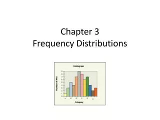
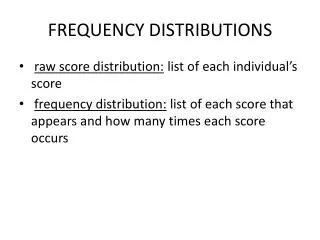
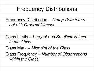
Frequency Distributions • Variability in an environmental variable results in frequency distribution of observed values • Frequency Distribution histogram: a type of graph that “bins” data into intervals to depict the distribution as a histogram (bar graph) • Provides a convenient way to look at the variability in the data • Example: data from an experimental set of ecosystem manipulations: values of water pH from wetlands with differing plant communities
The role of biodiversity in wetland ecosystem functioning Katia A. M. Engelhardt University of Maryland Center for Environmental Science Appalachian Laboratory
Monospecies: Long-leaved Courtesy Prof. Katia Engelhardt
Monospecies: Horned pondweed Courtesy Prof. Katia Engelhardt
Monospecies: Sago pondweed Courtesy Prof. Katia Engelhardt
Species mix: Community #1 Courtesy Prof. Katia Engelhardt
Collecting samples (note the comfortable chair) Courtesy Prof. Katia Engelhardt
In class illustration • Illustration of placing pH data into ‘bins’ for display using a histogram, resulting in a frequency distribution histogram
Using Histograms to graph data For the same data, histogram appearance will differ based on ‘bin size’. Example: pH in artificial wetland pools Data courtesy Dr. Katia Engelhardt
Brief review:Measures of central tendency and dispersion in data Central tendency: • Mean (average) • Median (middle point in ordered data) • Mode (most common value) Measure of dispersion: • Standard deviation (sd). Approx. 2/3 of the observations fall within plus or minus 1 sd of the mean.
Histogram with normal distribution superimposed Data courtesy Dr. Katia Engelhardt
Normal Distribution: • A commonly used model, or approximation, of frequency distributions of environmental data • Bell-shaped • Mean = median = mode • Standard deviation (SD) • In a dataset, measure of dispersion about the center • If normally distributed, 2/3 of observations lie within ± 1 SD of the mean • Not all data are normally distributed – the ‘normal’ curve is simply a widely used approximation that is often times a good one.
Source: Hornberger et al. 1998, Elements of Physical Hydrology
Frequency distributions Classification Frequency distributions are a good stepping stone to help us understand ‘Classification’ of data in a GIS for depiction in views and on layouts “Classification” • Pick a particular attribute or field, and choose how it will be displayed in the View • Involves choosing a ‘bin size’ and number of bins to categorize the data into
A View, Theme, and its Attribute Table in ArcView • One attribute table for each theme • In an attribute table, one row per feature (whether polygons, lines, or points) • Each Column in the table is an attribute, or field
The GIS links the spatial information of each feature in the theme with its data in the attribute table Foote & Huebner, The Geographer’s Craft, UC Boulder
Frequency distributions Classification Frequency distributions are a good stepping stone to help us understand ‘Classification’ of data in a GIS for depiction in views and on layouts “Classification” • Pick a particular attribute or field, and choose how it will be displayed in the View • Involves choosing a ‘bin size’ and number of bins to categorize the data into
Many decisions are made in classifying an attribute into categories for depiction • Are you (1) exploring & analyzing the data, or (2) trying to make a map? • If (1), what do you want to know? • If (2), what do you want to emphasize? • How many categories do you want to depict? • What rule do you want to use to divide the categories? • What color scheme suits your purposes? • Should ‘zero’ be its own category, or included in one of the others?
Classification: Natural Breaks (Jenk’s) Class breaks are set where there are ‘jumps’ in values Emphasizes natural groups of values – works better for some datasets than others. Works best for datasets with gaps in values or with clusters of values. Mitchell 1999, The ESRI Guide to GIS Analysis, Vol I
Classification: Quantile Class breaks are set so that each class contains an equal number of features Here the ‘features’ are polygons; but they could be streams, or streets, etc. Based on the percentile and median (50th percentile) concepts: with odd number of classes, the middle class will contain the median 4 classes = quartiles; 10 classes = deciles . . . Mitchell 1999, The ESRI Guide to GIS Analysis, Vol I
Classification: Equal Interval Class width, in values, is the same for every class Simply breaks the entire range into intervals of equal width. Emphasis on absolute differences. (With a uniform distribution, result would be about an equal number of features in each class.) Mitchell 1999, The ESRI Guide to GIS Analysis, Vol I
Classification: Standard Deviation GIS software calculates the mean and standard deviation of values, then sets class breaks as standard deviations from the mean Data need not be normally distributed to use this. Works best if your audience understands basic statistics. Note 3-color range used to show positive, middle, and negative (see Mitchell 1999) Mitchell 1999, The ESRI Guide to GIS Analysis, Vol I
Additional illustration of classification results • See the reading on Classification Methods – ESRI manual pdf
Lab this week: Classification of data in Census Blocks Human population
Introduction to Environmental AnalysisEnviron 239Instructor: Prof. W. S. Currie GSIs: Nate Bosch, Michele Tobias Skills Unit 2:Classifying and Depicting Data in a GIS: Second lecture
Normalizing data • Taking absolute numbers of a variable and dividing by another variable is called normalizing • Normalizing by area: • Dividing cancer cases in each township by the area of the township would produce cases / area • Normalizing by population: • Dividing cancer cases in each township by population would produce cases per capita. • Either of these is easily done in a GIS attribute table by creating a new, normalized field • Will do in lab this week: population density by census block
Illustration of classification and use of colors to depict spatial data: Nitrogen mineralization in forested land
Color choices you make in creating a depiction of spatial data Value Intensity (saturation) Hue
Illustration of the use of data resolution and color • Depiction of election results
Form small groups to discuss this: Suppose you worked for an environmental consulting firm that was hired to look into this, and this was your starting point. Looking at this map, what questions would you have? Cape Cod Times, 25 June 1995 -- Valiela 2001
Some possible questions • What does ‘elevations’ mean? • Where is the mean or median? In the ‘moderate elevations’ category? • Is the comparison just within Cape Cod, or compared to the rest of MA, or all the US? • What does ‘significant, moderate, lower’ mean? (And how were these categories classified?) • Do the data measure absolute numbers of cases? • Or density of cancer occurences per unit area, or cases per capita? • Were the data collected uniformly? • Could a pattern like this arise from random chance? • Are there likely variables, across space, that could prove explanative, and if so are there spatial correlations? • For example, what does a map of the retirement population look like?
Could a spatial pattern like this arise through random chance? • Out of 32 polygons: • 15 are light or dark grey; • 7 are dark grey
Could a spatial pattern like this arise through random chance? We will fill this in randomly.
Flip a penny 5 times and record the number of tails. We will fill in these colors randomly: • 0, 1, 2: white • 3: light grey • 4, 5: dark grey
I filled these in spatially using a random number generator, with: • White: below the mean • Light grey: above the mean • Dark grey: > 0.7 sd above the mean
This is the distribution that the class came up with last year (2005)
Additional illustration using frequency distribution histograms in a GIS Histograms are an important tool in GIS analysis • Frequency counts can be multiplied by areal cell size to provide an areal analysis
Urban Agriculture Hardwood forest Coniferous forest Mixed forest Tundra Water Wetland Cleared Bedrock Land Cover in White Mountain National Forest, NH Derived from Landsat Thematic Mapper, courtesy GRANIT project, Complex Systems Research Center, UNH
Area by forest type and elevation zone:as a frequency distribution Currie & Aber 1997, Ecology 78:1844-1860 Note unequal bin widths … WHY?