What is land-atmosphere feedback on precipitation?

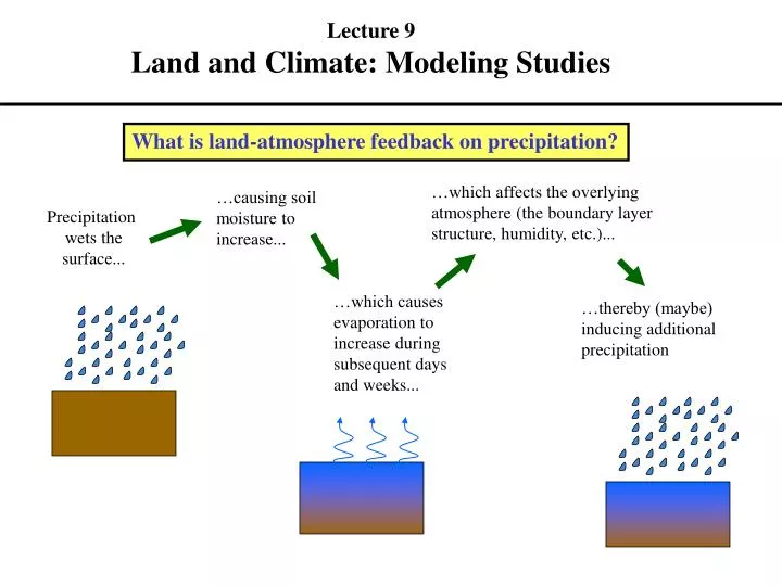
1. Lecture 9 Land and Climate: Modeling Studies What is land-atmosphere feedback on precipitation? …which affects the overlying atmosphere (the boundary layer structure, humidity, etc.)... …causing soil moisture to increase... Precipitation wets the surface... …which causes evaporation to increase during subsequent days and weeks... …thereby (maybe) inducing additional precipitation

2. Perhaps such feedback contributes to predictability. Short-term weather prediction with numerical models (e.g., those shown on the news every night) are limited by chaos in the atmosphere. Initialize model with that state; integrate into future Establish atmospheric state Short-term (~several days) weather prediction Decay reflects short timescale of atmospheric “memory” Relevance of initial conditions Atmosphere Sunday’s forecast for Tuesday (March 29, 2005): mostly sunny, high of 63F (17C). days

3. Relevance of initial conditions Ocean Land months For longer term prediction, we must rely on slower moving components of the Earth’s system, such as ocean heat content and soil moisture. Associated prediction of weather, if weather responds to these states Establish ocean state, land moisture state Initialize model with those states; integrate into future Long-term (~weeks to years) prediction of ocean and/or land states For soil moisture to contribute to precipitation predictability, two things must happen: 1. A soil moisture anomaly must be “remembered” into the forecast period. 2. The atmosphere must respond in a predictable way to the remembered soil moisture anomalies

4. Part 1: Soil Moisture Memory Observational soil moisture measurements give some indication of soil moisture memory. Vinnikov and Yeserkepova, 1991 Soil moisture timescales of several months are possible. “The most important part of upper layer (up to 1 m) soil moisture variability in the middle latitudes of the northern hemisphere has … a temporal correlation scale equal to about 3 months.” (Vinnikov et al., JGR, 101, 7163-7174, 1996.) Vinnikov and Yeserkepova, 1991

5. Delworth and Manabe (1988) analyzed soil moisture memory in the GFDL GCM and came up with a Markovian framework for characterizing it. We will discuss Delworth and Manabe’s soil moisture memory analysis further during the round-table discussion. D&M’s memory analysis was recently furthered at Goddard...

6. s s Koster and Suarez, 2001

7. Memory equation:

8. Seasonality term: swn/swn+1

9. Evaporation term: cRn/Cs (and equivalently, the runoff term: aPn/Cs)

10. (the covariance term)

11. This analysis allows us to examine soil moisture memory in terms of both large-scale forcing and inherent LSM behavior (e.g., through a and c terms, which describe the sensitivity of evaporation and runoff to soil moisture). The memory equation reduces to that of Delworth and Manabe under several simplifying assumptions.

12. Recent idealized experiment to analyze soil moisture memory (Sarith Mahanama, GSFC) -- A perpetual July experiment was performed to investigate the effect of precipitation and net radiation on soil moisture memory. Two different LSMs (the Mosaic LSM and the NSIPP-Catchment LSM) were given identical water holding capacities, vegetation type, soil type etc. and were forced under a variety of artificially generated climates. -- The imposed climates had: • average monthly precipitations ranging from 15 to 500mm • average monthly net radiation ranging from 20 to 400mm (Water equivalent) • -- Essentially, within the idealized framework, the intermodel differences of soil moisture memory result solely from intermodel differences in the sensitivity of evaporation and runoff to soil moisture variations. • -- A total of 400 different “climates” were imposed on each LSM. The simulation associated with each climate was a 200-month perpetual July simulation. Sub-monthly distributions of the variables followed those of the PILPS2c 1979-July forcing data for a chosen region.

13. Idealized Experiment to analyze soil moisture memory Autocorrelation of soil moisture (r) in different climates:

14. Idealized Experiment to analyze soil moisture memory Differences in autocorrelation of soil moisture (r) in different climates:

15. Superposition of ISLSCP-I July net radiation and precipitation on memory difference plot:

16. Supplemental analysis of globally simulated soil moisture memory with the two different models. When the Mosaic and Catchment LSMs are given the same soil moisture holding capacities, the Catchment LSM indeed shows higher memory for intermediate dryness index. When the Mosaic and Catchment LSMs are given their own, model-specific soil moisture holding capacities, the memory differences are seen to be largely a func-tion of the difference in capacity. (I.e., to some extent, a larger water holding capacity implies a larger memory.)

17. Effect of Climate Bias on Evaporative Regime Different sensitivities of evaporation to soil moisture result from different climatologies of forcing. Errors in memory due to AGCM biases in forcing

18. Part 2: Atmosphere’s Response to Soil Moisture Anomalies Three ways of looking for evidence of atmospheric response: 2. Simple analytical models. 3. AGCM studies. 1. Examine observational data. Very difficult. (See next lecture.) Advantage: feedbacks can be quantified and easily understood. Disadvantage: ignores some nonlinearities and complexities of system. Useful for several reasons: (a) full set of diagnostic out-puts, (b) inclusion of nonlinearities, and (c) ability to do sensitivity studies. Examples: Rodriguez-Iturbe et al., WRR, 27, 1899-1906, 1991. Brubaker and Entekhabi, WRR, 32, 1343-1357, 1996. Liu and Avissar, J. Clim, 12, 2154-2168, 1999.

19. AGCM evidence goes way back... Shukla and Mintz (1982) provide one of the first AGCM studies demonstrating the impact of land moisture anomalies on precipitation: Questions that can be addressed with an AGCM: How large is the impact of a land anomaly on the atmosphere? What are the relative roles of ocean variability, land variability, and chaotic atmospheric dynamics in determining precipitation over continents?

20. Studies examining the impact of “perfectly forecasted” soil moisture on the simulation of non-extreme interannual variations. Some examples: Delworth and Manabe, J. Climate, 1, 523-547, 1988. Dirmeyer, J. Climate, 13, 2900-2922, 2000. Round-table discussion See GSWP lecture Douville et al., J. Climate, 14, 2381-2403, 2001. Koster et al., J. Hydromet., 1,26-46, 2000. Dry conditions Wet conditions Simulations used: Ensemble 1: Sixteen 45-year simulations at 4oX5o with Interactive land surface processes Prescribed interannual-varying SST Ensemble 2: Sixteen 45-year simulations at 4oX5o with Fixed land surface processes (but with realistic interannual variations) Prescribed interannual-varying SST 1987 conditions 1988 conditions

21. Description of this last study... # of Total Exp. simulations Length years Description Evaporation efficiency (ratio of evaporation to potential evaporation) prescribed at every time step to seasonally-varying climatological means A 4 200 yr 800 AL 4 200 yr 800 AO 16 45 yr 720 ALO 16 45 yr 720 Prescribed, climatological land; climato- logical ocean Interactive land, climato- logical ocean Prescribed, climatological land, interan- nually varying ocean SSTs set to seasonally-varying climatological means (from obs) SSTs set to interannually-varying values (from obs) Interactive land, interan- nually varying ocean LSM in model allowed to run freely Koster et al., J. Hydromet., 1, 26-46, 2000

22. Analysis of the simulation output shows that land and ocean contribute differently to continental precipitation variability. Annual precipitation variances Seasonal precipitation variances (from a similar 1995 study)

23. Simulated precipitation variability can be described in terms of a simple linear system: Total precipitation variance Precipitation variance in the absence of land feedback s2ALO s2ALO= s2AO[ Xo + ( 1 - Xo ) ] s2AO Fractional contribution of ocean processes to precipitation variance Land-atmosphere feedback factor Fractional contribution of chaotic atmospheric dynamics to precipitation variance

24. Contributions to Precipitation Variability

25. More from Koster et al. (2001) In an additional ensemble, every member of the ensemble is subject to the same time series of evaporation efficiency. Does the precipitation respond coherently to this signal? Results for SST control over precipitation coherence: A variable W is defined that describes the coherence between the different precipitation time series.

26. Koster et al. (2001) (cont.) Boreal summer Boreal winter Results for SST and soil moisture control over precipitation coherence Differences: an indication of the impacts of soil moisture control alone

27. Koster et al. (2001) (cont.) Why does land moisture have an effect where it does? For a large effect, two things are needed: a large enough evaporation signal a coherent evaporation signal – for a given soil moisture anomaly, the resulting evaporation anomaly must be predictable. Both conditions can be related to relative humidity: The dots show where the land’s signal is strong. From the map, we see a strong signal in the transition zones between wet and dry climates. Evap. coherence

28. Why does land-atmosphere feedback occur where it does? One control: Budyko’s dryness index variance amplification factor

29. The results of this study could be highly model-dependent. Here are the results from another study, using the COLA GCM: Blue shading indicates regions where a continually prescribed soil wetness has a direct impact, through evaporation, on precipitation simulated during boreal summer in a climate model. Percentages indicate the likelihood that simulated impacts are not the product of chance. Some critical questions: 1. How does the atmosphere’s response to soil moisture anomalies vary with AGCM? 2. Can we define an objective way of comparing this response? We address these questions with...

30. time step n time step n Part 1: Establish a time series of surface conditions (Simulation W1) time step n+1 Step forward the coupled AGCM-LSM Step forward the coupled AGCM-LSM time step n+1 Write the values of the land surface prognostic variables into file W1_STATES Write the values of the land surface prognostic variables into file W1_STATES Step forward the coupled AGCM-LSM Step forward the coupled AGCM-LSM Throw out updated values of land surface prognostic variables; replace with values for time step n from file W1_STATES Throw out updated values of land surface prognostic variables; replace with values for time step n+1 from file W1_STATES (Repeat without writing to obtain simulations W2 – W16) … the GLACE Experiment Coupled large scale GLACE is a follow-on to a pilot coupled model intercomparison experiment. (K02: Koster et al., Comparing the degree of land-atmosphere interaction in four atmospheric general circulation models, J. Hydromet., 3, 363-375, 2002.) Part 2: Run a 16-member ensemble, with each member forced to maintain the same time series of surface prognostic variables (Simulations R1 – R16) Part 3: Same as Part 2, but only reset the deep soil moisture variables. (some slides are from Z. Guo)

31. How does GLACE build on K02? Participation from a wider range of models. The idea is to generate a comprehensive “table” of coupling strengths, a table that can help in the interpretation of the published results of a wide variety of models. Separation of the effects of “fast” and “slow” reservoirs. The K02 results largely reflect the specification of the “fast” reservoirs (e.g., surface temperature). They thus may have little relevance to issues of seasonal prediction. Effect on air temperature. Ignored in the K02 study is the effect of the specification of surface variables on the evolution of air temperature. (This is a particularly interesting issue when only the “slow” soil moisture reservoirs are specified.) Correction of miscellaneous technical issues. Lessons learned from the K02 study can be applied immediately to GLACE.

32. Participating Groups Model Contact Status 1. BMRC with CHASM McAvaney/Pitman submitted 2. U. Tokyo w/ MATSIRO Kanae/Oki submitted 3. COLA with SSiB Dirmeyer submitted 4. CSIRO w/ 2 land schemes Kowalczyk submitted 5. NCAR submitted 6. Env. Canada with CLASS Verseghy submitted 7. GFDL with LM2p5 Gordon submitted 8. GSFC(GLA) with SSiB Sud submitted 9. Hadley Centre w/ MOSES2 Taylor submitted 10. NCEP/EMC with NOAH Lu/Mitchell submitted 11. NSIPP with Mosaic Koster submitted 12. UCLA with SSiB Xue submitted

33. All simulations in ensemble respond to the land surface boundary condition in the same way W is high Simulations in ensemble have no coherent response to the land surface boundary condition W is high 6-day averages used in GLACE

34. Seasonality in SSTs, solar variability, etc., leads to some coherence amongst ensemble members Example at one CCSR grid cell Subtracting W for ensemble R or ensemble S from that for ensemble W isolates the land’s impact on precipitation coherence. The land’s impact is larger when all surface variables are prescribed (ensemble R) rather than just the subsurface soil moisture (ensemble S).

35. Ωp (S - W): Impact of sub-surface soil moisture on precipitation GFDL COLA UCLA GFDL COLA UCLA HadAM3 BMRC NCEP HadAM3 BMRC NCEP CCCma NSIPP CSIRO-CC3 CCCma NSIPP CSIRO-CC3 NCAR GEOS CCSR/NIES CSIRO-CC4 GEOS

36. The GLACE project showed that while the 12 participating models differ in their land-atmosphere coupling strengths, certain features of the coupling patterns are common to many of the models. These features are brought out by averaging over all of the model results:

37. Precipitation hotspots Air temperature hotspots Average over all models Average over all models Average over 8 “best” models, based on comparison at each point w/observed precipitation. Average over 8 “best” models, based on comparison at each point w/observed precipitation.

38. What defines the coupling strength within a given model? It’s helpful to consider coupling in terms of a two-part process: 1. Soil moisture variations lead to variations in evaporation, a proxy for the full surface energy budget. 2. Evaporation variations lead to variations in precipitation. precipitation variations evaporation variations soil moisture variations

39. To quantify the first process, we use a diagnostic that characterizes the nature of the evaporation signal: sE * (WE(S) – WE(R)) Rationale: The atmosphere is more likely to produce a coherent response to the land surface if the signal it sees at the surface is itself large and coherent. HIGH VALUE OF DIAGNOSTIC: LOW VALUE OF DIAGNOSTIC: E variability high and coherence high E variability low, coherence low E variability high, coherence low E variability low, coherence high

40. The diagnostic indeed explains much of the intermodel difference in coupling strength. For example, it explains about 60% of the inter-model differences in the Great Plains. The other 30% results from differ-ences in atmospheric parameterization (e.g., convection), sampling error, etc. coupling strength sE * (WE(S) – WE(W))

41. Global averages The two factors in the diagnostic, sEandWE(S) – WE(W), can be examined separately. (Evap. variability) (Evap. coherence) WE(S) – WE(W) Coupling strength for BMRC is low due to low evaporation variability Coupling strength for GFS/OSU is low due to low evaporation coherence sE

42. efficient transmission The evaporation signal is transmitted into precipitation via various parameterizations of atmospheric processes signal transmission (second process: evaporation affects precipitation) strong signal weak signal signal in evaporation (first process: soil moisture affects evaporation) inefficient transmission

43. coupling strength and AGCM parameterizations Evap formulations in these three models might not favor the coupling between sub-surface soil moisture and surface moisture fluxes

44. coupling strength and AGCM parameterizations Global averages coupling between surface fluxes and precipitation is mostly via convective precipitation scheme in the AGCMs LP CP TP Global averages

45. Experiment website: http://glace.gsfc.nasa.gov

46. How about AGCM studies that only initialize the soil moisture? (I.e., studies that don’t prescribe soil moisture throughout the simulation period?) Such studies include Oglesby and Erickson, J. Climate, 2, 1362-1380, 1989. Also: Beljaars et al., Mon. Weather Rev., 124, 362-383…. Wet initial- ization Rind, Mon. Weather Rev., 110, 1487-1494. June 1 initialized dry Dry initial- ization Differ- ences

47. Impact of Soil Moisture Predictability on Temperature Prediction (darker shades of green denote higher soil-moisture impact) …and a study by Schlosser and Milly (J. Hydromet., 3, 483-501, 2002), in which the divergence of states in a series of parallel simulations was studied in detail: Predictability Timescale Estimate (via memory) for soil moisture Actual Predictability Timescale (diagnostics of precipitation show a much weaker soil-moisture impact) Some recent studies have examined the impact of soil moisture initialization on forecast skill (relative to real observations). These will be discussed in the next lecture.