Download
1 / 37
370 likes | 525 Views
Wide field imaging Non-copalanar arrays. Kumar Golap Tim Cornwell. Goals of astronomical imaging. To recover the most faithful image of the sky Try to get the best signal to noise possible Reduce distortion as far as possible . Overview. Problems with imaging with non-coplanar arrays

E N D
Wide field imagingNon-copalanar arrays Kumar Golap Tim Cornwell Non-coplanar arrays
Goals of astronomical imaging • To recover the most faithful image of the sky • Try to get the best signal to noise possible • Reduce distortion as far as possible Non-coplanar arrays
Overview • Problems with imaging with non-coplanar arrays • 3D-imaging • Wide-field imaging • ‘w’ term issue • When we have to deal with this problem • Why it occurs and its effects • Some solutions • Related issues Non-coplanar arrays
What is the ‘w’ term problem • The relationship between visibility measured and Sky Brightness is given by the equation below. • It is not straight forward to invert and is NOT a Fourier transform • is a 3-D function while is only a 2-D function • If we take the usual 2-D transform of the left side…the third variable manifests itself when the ‘w’ becomes large. Non-coplanar arrays
Some basic questions? • When ? : Imaging at low frequency (1.4, 0.3, 0.075 GHz with VLA) • Field of view ~ many degrees • Sky filled with mostly unresolved sources • e.g. For VLA at 0.3 GHz, always 1 Jy point source, and > 12Jy total • Also Galactic plane, Sun, bright sources (cygnus-A, Cas-A) • Why ? Simple geometric effect: The apparent shape of the array varies across the field of view • Why bother ? : Because it violates the basic aims of imaging • Imaging weak sources in presence of diffraction patterns • e.g. < 1 mJy/beam at 0.3 GHz • Imaging extended emission • e.g. Galactic center at 0.3 GHz Non-coplanar arrays
An example of the problem • Image on the left is done with ‘2d’ imaging and the one on the right shows what the region should look like. The region is away from the pointing center of the array Non-coplanar arrays
An example of the problem • Image of an SNR near the Galactic center while ignoring and not ignoring the ‘w’ term. Non-coplanar arrays
A demonstration • Response to a point source at various places in the field of view if we were to image as using the usual ‘2D’ transform method. Non-coplanar arrays
Formal description • For small fields of view, the visibility function is the 2-D Fourier transform of the sky brightness: • For large fields of view, the relationship is modified and is no longer a 2-D Fourier transform Non-coplanar arrays
Projection • Must represent celestial sphere via a projection • Interferometers naturally use “sine” projection • Direction cosines: • Distance AA’: Non-coplanar arrays
Point source • Consider a point source of flux at • The “extra” phase is given by AA’ multiplied by • Area projection term: Non-coplanar arrays
Analysis of effects • Phase error in neglecting non-coplanar term: • Require maximum baseline B and antenna diameter D • Or Clark rule: (Field of view in radians).(Field of view in beams) <<1 Non-coplanar arrays
Effect on noise level • If nothing is done, side-lobes of confusing sources contribute to the image noise • Quadratic sum of side-lobes due to source counts over antenna primary beam Non-coplanar arrays
Noise achieved v/s Field of view cleaned Non-coplanar arrays
Coplanar baselines • There is a special case of considerable interest: coplanar baselines: • By redefining the direction cosines we can derive a 2D Fourier transform: • Using a simple geometric interpretation: a coplanar array is stretched or squeezed when seen from different locations in the field of view • Conversely: a non-coplanar array is “distorted” in shape when seen from different locations in the field of view Non-coplanar arrays
A simple picture: Planar array • Different points in the sky see a similar array coverage except compressed by the term ‘l’ Non-coplanar arrays
A simple picture: non planar array Non-coplanar arrays
Coplanar baselines • Examples: • East-West array • can ignore this effect altogether for EW array • VLA for short time integration • can ignore for sufficiently short snapshot Non-coplanar arrays
Possible solutions: 3D Fourier transform • Can revert to Fourier transform by embedding in a 3D space • Brightness defined only on “Celestial Sphere”: • Visibility measured in space • All 2D deconvolution theory can be extended straightforwardly to 3D • Solve 3D convolution equation using any deconvolution algorithm but must constrain solution to lie on celestial sphere Non-coplanar arrays
Explanation of 3-D transform • 3-D Fourier transform of the sampled Visibility leads to the following ‘image volume’ function: • This has meaning on the surface of but we have to do a 3-D deconvolution which increases the number of points visibility a large factor. Non-coplanar arrays
Possible solutions: Sum of snapshots • Decompose into collection of snapshots, each with different effective coordinate systems • Two approaches for deconvolution: • Treat each image as independent: • Easy but each snapshot must be deconvolved separately • Derive each image from a “master” image: • Expensive computationally, since the coordinate conversions take a considerable amount of time Non-coplanar arrays
Picture of the different coordinate systems for different snapshots • 2 different snapshots array positions appear planar in very different directions. Non-coplanar arrays
Possible solutions: Faceted transform • Decompose into summation of the visibilities predicted from a number of “facets”: • Where the visibility for the k th facet is: The apparent shape of the array is approximately constant over each facet field of view Non-coplanar arrays
Possible solutions: PSF interpolation in a image plane deconvolution • The facet size can be made very small, tending to a pixel. This makes a dirty image with the ‘w’ induced PHASE term corrected for. So image is not dephased. But the ‘uv’ projection is not self-similar for different directions, which implies that the PSF shape is a function of position. • The technique involves estimating PSF’s at different positions and then interpolating in between when deconvolving in the image plane. Non-coplanar arrays
Varying PSF • Even though in the ‘facetted’ and ‘interpolation’ method the dephasing due to the ‘w’ is corrected for. The different uv coverage still remains. We still need a position dependent deconvolution. • The following demonstration shows the PSF (at different point in the field of view) difference from the one in the direction of the pointing center. This difference is after the correcting for the phase part of the `w’ effect. Non-coplanar arrays
PSF difference Non-coplanar arrays
Overview of possible solutions Non-coplanar arrays
Faceted transform algorithm • Used in AIPS IMAGR task, AIPS++ imager, dragon tools • Iterative, multi-stage algorithm • Calculate residual images for all facets • Partially deconvolve individual facets to update model for each facet • Reconcile different facets • either by cross-subtracting side-lobes • or by subtracting visibility for all facet models • Recalculate residual images and repeat • Project onto one tangent plane • image-plane interpolation of final cleaned facets • (u,v) plane re-projection when calculating residual images Non-coplanar arrays
Reconciling Facets to single image • Facets are projected to a common plane. This can be done in image plane (in AIPS, flatn). • Re-interpolate facet image to new coordinate systems • Cornwell and Perley (1992) • or in equivalently transforming the (u,v)’s of each facet to the one for the common tangent plane (in AIPS++) • Re-project (u,v,w) coordinates to new coordinate systems during gridding and de-gridding • Sault, Staveley-Smith, and Brouw (1994) Non-coplanar arrays
Number of facets • To ensure that all sources are represented on a facets, the number of facets required is (Chap 19) ~ • Worst for large VLA configurations and long wavelengths • More accurate calculation: • Remove best fitting plane in (u,v,w) space by choosing tangent point appropriately • Calculate residual dispersion in w and convert to “resolution” • Derive size of facet to limit “peeling” of facet from celestial sphere • Implemented in AIPS++ imager tool via function “advise” Non-coplanar arrays
An example Non-coplanar arrays
An iterative widefield imaging/self-cal routine: An AIPS++ implementation in dragon • Setup AIPS++ imager for a facetted imaging run with outlier fields (or boxes) on known strong confusing sources outside mainlobe • Make a first Image to a flux level where we know that the normal calibration would start failing • Use above model to phase self calibrate the data • Continue deconvolution from first image but with newly calibrated data to a second flux level. Repeat the imaging and self cal till Amplitude selfcal is needed… then do a simultaneous amplitude and Phase self cal. • Implemented as a glish script. Non-coplanar arrays
Example of a dragon output: Non-coplanar arrays
Other related issues with widefield imaging apart from ‘w’ • Bandwidth decorrelation: • Delay across between antennas cause signal across the frequency band to add destructively • Time average smearing or decorrelation (in rotational synthesis arrays only) • Change in uv-phase by a given pair of antennas in a given integration time • If imaging large structures proper short spacing coverage or mosaicing if necessary (more on this in the next talk by Debra Shepherd) • Missing short spacing causes negative bowl and bad reconstruction of large structures Non-coplanar arrays
Other related issues with widefield imaging apart from ‘w’…cont’d • primary beam asymmetry: • Sources in the outer part of the primary beam suffers from varying gains (and phases) in long track observations. This may limit the Signal to noise achievable. If model of the beam is known it can be used to solve for the problem. Else can be solved for as a direction phase dependent problem as mentioned below. • Non isoplanaticity: • Low frequency and long baselines problem. The 2 antennas on a baseline may see through slightly different patches of ionosphere. Cause a direction dependent phase (and amplitude) error. Can be solved for under some restraining conditions (More on this in Namir Kassim’s talk). Non-coplanar arrays
Summary • Simple geometric effect due to non-coplanarity of synthesis arrays Apparent shape of array varies across the field of view • For low frequency imaging with VLA and other non-coplanar arrays, will limit achieved noise level • Faceted transform algorithm is most widely used algorithm • AIPS: IMAGR task • AIPS++: imager (version for parallel computers available), dragon tools • Processing: • VLA mostly can be processed on typical personal computer • A-configuration (74MHz) and E_VLA needs parallelization Non-coplanar arrays
Bibliography • Cornwell, T.J., and Perley, R.A., “Radio interferometric imaging of large fields: the non-coplanar baselines effect”, Astron. & Astrophys., 261, 353-364, (1992) • Cornwell, T.J., “Recent developments in wide field imaging”, VLA Scientific Memorandum 162, (1992) • Cornwell, T.J., “Improvements in wide-field imaging” VLA Scientific Memorandum 164, (1993) • Hudson, J., “An analysis of aberrations in the VLA”, Ph.D. thesis, (1978) • Sault, R., Staveley-Smith, L., and Brouw, W.N., Astron. & Astrophys. Suppl., 120, 375-384, (1996) • Waldram, E.M., MCGilchrist, M.M., MNRAS, 245, 532, (1990) Non-coplanar arrays