Download
1 / 63
850 likes | 1.88k Views
Hierarchical Routing:. Leonard Kleinrock and Farouk Kamoun : Hierarchical routing for large networks: Performance evaluation and optimization, Computer Networks, Vol. 1(3 ):155 - 174, , Jan. 1977.

E N D
Hierarchical Routing: Leonard Kleinrock and Farouk Kamoun: Hierarchical routing for large networks: Performance evaluation and optimization, Computer Networks, Vol. 1(3):155-174, , Jan. 1977. PNNI Routing, Private Network-Network Interface Specification Version 1.0, ATM Forum, March 1996. Paul Tsuychia, The Landmark Hierarchy: A new hierarchy for routing in very large networks, ACM Sigcomm, p. 35-42, 1988.
Leonard Kleinrock and Farouk Kamoun:Hierarchical routing for large networks Performance evaluation and optimizationComputer Networks, Vol. 1(3), Jan 1977, pp. 155-174 (uses slides prepared by Boris Drazic)
Routing in the 1970s • Computer networks are new and have a small number of nodes • ARPANET is predecessor of Internet • Uses concepts of: • routing table (RT) • Distributed routing protocols ARPANET 1969
Routing in the 1970s • Computer networks are new and have a small number of nodes • ARPANET is predecessor of Internet • Uses concepts of: • routing table (RT) • Distributed routing protocols ARPANET 1971
Routing in the 1970s • Computer networks are new and have a small number of nodes • ARPANET is predecessor of Internet • Uses concepts of: • routing table (RT) • Distributed routing protocols • One routing table for each “node” of the network ARPANET 1980
Number of Internet Hosts Source: Internet Systems Consortium (www.isc.org)
Active BGP Entries (FIB) Source: http://www.cidr-report.org/
Example of Routing Table (1) Routing table for node a
Hierarchical Routing Schemes • Goal: Reduce the size of routing tables (RT) • Approach: Keep complete routing information about nodes that are “close” and less information about nodes that are “far away” • One RT entry for every destination that is “close” • One RT entry for every set of destinations that is “far away” • Forwarding has two parts: • Forward the message “close” to the destination • Forward the message to the destination
Example of RT (2) Routing table for node a “far away” destinations “close” destinations `
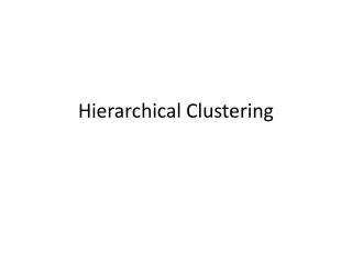
m-level Hierarchical Clustering • Create a hierarchy with m levels by: • Each node is a 0th level cluster • Group nodes into 1st level clusters • Group 1st level clusters into 2nd level clusters • …
3rd level cluster 2nd level cluster 1st level cluster 0th level cluster `
3rd level cluster 2nd level cluster 1st level cluster 0th level cluster `
RT in 3-level Hierarchical Clustering nodes in same cluster 0th level cluster entries 1st level cluster entries clusters in same supercluster 2nd level cluster entries superclusters `
Forwarding Rules: Forward to leftmost cluster in address; When reached, forward to next cluster to the right in the address Example: Source: 1.1.1 Destination: 3.2.2
What is the optimal clustering in a network with N nodes? • Proposition 1: Given the number of levels m, if each cluster has the same number of lower level clusters, the minimum routing table lengths is . • Proposition 2: The global optimal clustering is achieved for m=ln(N), when each cluster has e lower level clusters, and the minimum table length is l=eln(N).
Minimum Relative Table Length RT size decreases fast for m < ln(N) Minima for: m= ln(N)
Hierarchical Routing increases path length Example: Source: a Destination: i Shortest path: 4 hops With hierarchical routing: 5 hops
Increased Path Length • Assumption 1: Every cluster has the same number of sub-clusters and for every pair of nodes in a cluster a path exists between them in that cluster • Assumption 2: The diameter of any kth level cluster is less or equal to some quantity dk • hc is average path length with clustering • h is average path length without clustering
Increased Path Length • Proposition 10: Under Assumptions 1 and 2
Limiting Performance • Assumption 3: Any cluster contains the shortest path between any pair of nodes that belong to that cluster • Proposition 11: Under Assumptions 1-3, for an m-level optimal clustering hierarchy where the diameter of any cluster is bounded by a power law function of the number of nodes in that cluster:
Increased Path Length • Define as the increase in path length produced by introducing clustering • Observe E, which is a bound on D • Presented results for a network where Assumptions 1-3 hold
Decrease in RT Length for a Given Maximum Increase in Path Length Interpret “E” as the tolerated “stretch” factor
Conclusion • In very large networks, hierarchical routing schemes achieve great reduction of routing table size with only a small increase in path lengths between nodes, when compared to non-hierarchical routing schemes
Hierarchical Routing Application: ATM NetworksIn the 1990s, the ATM Forum adopted a routing scheme which is based on hierarchical routing
ATM Connection Acronyms • VC - virtual channel, synonymous with “circuit” or “connection” • VPC - virtual path connection • VCC - virtual channel connection • PVC - permanent virtual circuit • PVP - permanent virtual path • SVC - switched virtual circuit • SVP - switched virtual path • SPVC - switched/signaled/soft permanent virtual circuit • PMP - point-to-multipoint
Traditional Network Infrastructure Telephone network Company B Company A Data network Video network Residential user x
The B-ISDN vision (from mid 1980s!) BroadbandIntegrated Services Network (B-ISDN) Company B Company A Residential user x
ATM’s Key Concepts • ATM uses Virtual-Circuit Packet Switching • ATM can reserve capacity for a virtual circuit. This is useful for voice and video, which require a minimum level of service • Overhead for setting up a connection is expensive if data transmission is short (e.g., web browsing) • ATM packets are small and have a fixed sized • Packets in ATM are called cells • Small packets are good for voice and video transmissions Header(5 byte) Data (48 byte) Cell is 53 byte long
Virtual Paths and Virtual Circuits Link Virtual ChannelConnection Virtual Path Connections VPI identifies virtual path (8 or 12 bits) VCI identifies virtual channel in a virtual path (16 bits)
VPI/VCI assignment at ATM switches 1/24 3/24 7/24 2/17 3/24 1/40
PNNI UNI: User-to-Network Interface NNI: Network-to-Network Interface PNNI: Suite of protocols for topology discovery and routing of an ATM network
PNNI Routing • Goal of PNNI Routing: Establish a switching path from sender to receiver • PNNI characteristics: • Link State Routing • Source Routing • Hierarchical Routing • Crankback • Routing protocol information is sent on VPI/VCI=0/18
Link State Routing Algorithm • PNNI uses link state routing: • Each node floods route messages on its links to all nodes in the network • Each node has complete topology information • Source routing:PNNI computes route at the first switch • QoS:Route messages also contain QoS information on links • Hierarchy:PNNI deals with complex networks by using a hierarchy B.1.1 B.1.2 B.3.1 B.3.2 B.2.2 B.2.1 B.2.3
PNNI Routing Hierarchy B B.1 A • Routing hierarchy is defined recursively: • Neighbor nodes build Peer Groups by comparing their address prefixes (nodes with longest prefix match are in the same peer group) • Each group behaves like a Logical Group Node (LGN) in the next level peer group C A.1 A.2 B.1.1 B.1.2 A.1.1 B.3.1 A.2.1 C.1.1 A.1.2 A.2.2 A.2.3 B.3.2 C.1.2 B.3 C.1 B.2.2 B.2.1 B.2.3 B.2
Building the PNNI Routing Hierarchy • Each switch is initialized with a 20-byte ATM address B.1.1 B.1.2 A.1.1 B.3.1 A.2.1 C.1.1 A.1.2 A.2.2 A.2.3 B.3.2 C.1.2 B.2.2 B.2.1 B.2.3
B.1 A.1 A.2 B.3 C.1 B.2 PNNI Routing Hierarchy • Nodes with common prefix A.1, A.2, B.2, B.2, B.3, C.1 each form a logical group node B.1.1 B.1.2 A.1.1 B.3.1 A.2.1 C.1.1 A.1.2 A.2.2 A.2.3 B.3.2 C.1.2 B.2.2 B.2.1 B.2.3
B B.1 A C A.1 A.2 B.3 C.1 B.2 PNNI Routing Hierarchy • Nodes with common prefix A, B, C each form a logical group node at the next level B.1.1 B.1.2 A.1.1 B.3.1 A.2.1 C.1.1 A.1.2 A.2.2 A.2.3 B.3.2 C.1.2 B.2.2 B.2.1 B.2.3
Resulting Hierarchy B B.1 A • Within each peer group, nodes or LGNs elect a peer group leader (PGL), which represents the peer group at the next level C A.1 A.2 B.1.1 B.1.2 A.1.1 B.3.1 A.2.1 C.1.1 A.1.2 A.2.2 A.2.3 B.3.2 C.1.2 B.3 C.1 B.2.2 B.2.1 B.2.3 B.2
Complete Hierarchy A C B B.1 A.1 A.2 C.1 B.3 B.2
Routing Messages Hierarchy Routing messages are called PNNI Topology State Packets (PTSP) • Nodes within each peer group exchange PTSP • Group Leader relays routing information from higher level topology to lower layer A C B B.1 A.1 A.2 C.1 B.3 B.2
Resulting Hierarchy B • Node B.2.3’s view of the network topology • Node can now run source routing C B.1 C B.3 A B.2.2 B.2.1 B.2.3 B.2
Source routing in the hierarchy A A.2 B A.1 B.2 A.1.1 A.2.3 A.2.1 desti-nation B.1 A.1.2 B.3 A.2.2 source • At A.1.1 : Route = [ (A.1.1, A.1.2), (A.1, A.2), (A, B)] • At A.1.2 : Route = [ (A.1, A.2), (A, B)] • At A.2.1 : Route = [ (A.2.1, A.2.2, A.2.3), (A.1, A.2), (A, B)] • At A.2.2 : Route = [ (A.2.1, A.2.2, A.2.3), (A.1, A.2), (A, B)] • At A.2.3 : Route = [ (A, B)] • At B.1: Route = [ (B.1, B.3), (A, B) ] • At B.3: Route = [ ]
Crankback and Alternate routing A A.2 B A.1 B.2 A.1.1 A.2.3 A.2.1 desti-nation B.1 A.1.2 B.3 A.2.2 QoS cannot be satisfied source • At A.1.1 : Route = [ (A.1.1, A.1.2), (A.1, A.2), (A, B)] • At A.1.2 : Route = [ (A.1, A.2), (A, B)] • At A.2.1 : Route = [ (A.2.1, A.2.2, A.2.3), (A.1, A.2), (A, B)] • At A.2.2 : Route = [ crankback: (A.2.1, A.2.2, A.2.3) , (A.1, A.2), (A, B)] • At A.2.1 : Route = [ (A.2.1, A.2.3), (A.1, A.2), (A, B)] • At A.2.3 : Route = [ (A, B)] • and so on
Paul Tsuychia: The Landmark Hierarchy: A new hierarchy for routing in very large networks ACM Sigcomm 1988, p. 35-42
Drawback of Hierarchical Routing Route from 3.2.1 1.2.3 Shortest path: 3.2.12.2.3 3.2.1 Hierarchical Route: 3.2.1 Area 3.1 Area 3.1 Area 1(Area 1.1) Area 1.1 Area 1.2(1.2.1) 1.2.1 1.2.2 1.2.2 1.2.3 1.2.2 1.2.1
Enter “Landmarks” • Landmarks can be seen from far away! • Landmark router: Normal router can see a landmark router from several hops away Information about landmark routers is disseminated to normal routers
Landmark router • Router 1 is landmark router with radius 2 • Routers up to 2 hops away have routing entries for Router 1 Router 1 can be seen from 2 hops away
Hierarchy of Landmarks Notation: i : level number (0 is lowest level, H is highest level) LMi: landmark at level-i LMi[id]: specific landmark at level iwith identifier id ri[id]: Radius of LMi[id] • Every router is a level-0 landmark with a small radius • Some level-0 landmarks are level-1 landmarks • Radius of level-1 landmark is greater than that of level-0; • Each level-0 landmark LM0 [id] can reach at least one level-1 landmark in r0[id]hops • Some level-1 landmarks are level-2 landmarks • Radius of level-2 landmark is greater than that of level-1; • Each level-1 landmark LM1 [id] can reach at least one level-11 landmark in r1 [id] hops …… • A small number of routers are level-H landmarks (“global landmarks”) • Every router “can see” all level-H landmarks