Download
1 / 1
10 likes | 143 Views
Genetic Algorithm The genetic algorithm starts with an initial population of protein conformations. The population numbers vary depending on the preference of the researcher. After the initial population has been determined, a potential energy function is applied to the population .

E N D
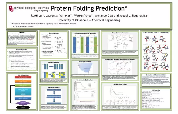
Genetic Algorithm • The genetic algorithm starts with an initial population of protein conformations. The population numbers vary depending on the preference of the researcher. • After the initial population has been determined, a potential energy function is applied to the population. • The reproduction process takes place with the occurrence of three genetic operators. Operators are rules that modify individuals and the population to include diversity to the process. • Selection – elitism within population • Crossover – exchange dihedral angles between chromosomes • Mutation – randomly replace a gen with a new one • Adaptation – maximize the fitness of each individual • The GA stops on the occurrence of or two occasions one is that there is a solution or the GA has proved the impossibility of the reproduction. Protein Folding Prediction* Rufei Lu**, Lauren M. Yarholar**, Warren Yates**, Armando Diaz and Miguel J. Bagajewicz University of Oklahoma ― Chemical Engineering *This work was done as part of the capstone Chemical Engineering class at the University of Oklahoma **Capstone undergraduate students Adaptation Operator Local Minimum Structures Energy Function α-helix/b-sheet Modified Operators • Abstract • The search for an efficient protein conformation predicting method began in 1972; however, only minor progress has been made towards the 3-D prediction algorithm. Our research focuses on a novel search and optimization method based on the concept of natural selection, a Genetic Algorithm. We have successfully developed a GA program (Genetic Algorithm based Protein Structure Search, GAPSS) that minimizes the potential energy of proteins and generates the corresponding Cartesian coordinates. We were also able to visualize the predicted conformations and compare them to their known natural conformations. • Conclusion and Recommendations • GAPPS predicts short isolated native protein structures accurately. • GAPSS has demonstrated its ability to determine natural conformations for unknown proteins. • The resolution and accuracy of GAPSS depends largely upon the fitness function and the GA parameters optimization process. • To further improve the method, a more refined fitness function with torsion angle penalty terms, bond stretching, and bond angle bending should be used. • Solvation energies and entropic effects need to be added. GAPSS predicted Single AA Conformations • 3 Primary Energy: • Electrostatic • Non-bonded (6-12) • Hydrogen-Bonded • “Torsion Energy “ ignored • Not real interaction • energy • Only introduces a penalty for positive torsion • Cysteine Loop-Closing • Introduced only when more than one cysteine is present in the protein Asparagine/N/Asn Aspartic Acid/D/Asp Alanine/A/Ala Set GA Parameters - - - Glycine/G/Gly Glutamic Acid/E/Glu Glutamine/Q/Gln Cysteine/C/Cys Initial Population Figure 1. Adaptation Operators. Linear gradient search on each chromosome to minimize energy. Fitness Function Methionine/M/Met Isoleucine/I/Ile Leucine/L/Leu Figure 2. Potential energy profile of best prediction run (initial population: 50; generation limits: 15, and mutation percentage: 90%): the structures at each point are displayed under the chart. The energy trend suggests that more stringent GA parameter might lead to lower energy. Figure 1. Modified Operators. (a) Crossover: Creates α-helices and b-sheets of random lengths at random start positions. Crossover will involve trading the two parameters between two individuals; (b) Mutation: Only circled region is only susceptible to mutation. Reproduction Process: Selection Crossover Mutation Adaptation Comparison of Predicted and Theoretical Enkephalin Threonine/T/Thr Serine/S/Ser Valine/V/Val Crossover Operator Offspring Generation Termination Criterion GAPSS Flow Chart Figure 5. Mutation Operators. (a) Uniform Mutation operator randomly replaces original values with values ranging from -180 to 180; (b) Non-uniform Mutation operator randomly replaces the value with different degrees. - GA Parameter Optimization End GA Potential Energy Profile Figure 1. Crossover Operators. (a) Random 2-point crossover operator randomly exchange between parents 2 angels at a time; (b) Multiple entries crossover operator applies multiple random exchanges along the chromosome Mutation Operator Bibliography A. LIWO, P. M., Wawak, R. J., Rackovsky, S., & Scheraga, H. A. (1993).Agostini, L., & Morosetti, S. (2003). Cox, G. A., Mortimer-Jones, T. V., Taylor, R. P., & Johnston, R. L. (2004). Creighton, T. E. (1988). Cui, Y., Chen, R. S., & Wong, W. H. (1998). Dandekar, T., & Argos, P. (1994). Dill, K. A. (1990). Gibson, K. D., & Scheraga, H. A. (1967). Gordon, M. S. (1969). Jayaram, B., Bhushan, K., Shenoy, S. R., Narang, P., Bose, S., Agrawal, P., et al. (2006). Klepeis, J. L., & Floudas, C. A. (1999). Momany, F. A., Carruthers, L. M., McGuire, R. F., & Scheraga, H. A. (1974). Momany, F. A., McGuire, R. F., Burgess, A. W., & Scheraga, H. A. (1975). Nemethy, G., Gibson, K. D., Palmer, K. A., Yoon, C. N., Paterllini, G., Zagari, A., et al. (1992). Pedersen, J. T., & Moult, J. (1996). Pedersen, J. T., & Moult, J. (1997). Pitzer, R. A. (1983). Rabow, A. A., & Scheraga, H. A. (1996). Sippl, M. J., Nemethy, G., & Scheraga, H. A. (1984). Standley, D. M., Gunn, J. R., Friesner, R. A., & McDermott, A. E. (1998). Unger, R., & Moult, J. (1993). Yan, J. F., Momany, F. A., & Scheraga, H. A. (1969). Yang, Y., & Liu, H. (2006). Figure 6 Performance analysis. (a) The minimum energy of each generation with different initial population at 3 generation limit and 20% mutation; (b) The minimum energy of each generation with different the percentage of mutation at 10 generation limit and 20 initial population. Figure 4. Comparisons of two predicted backbone structures with theoretical structure. (a) and (d) are the theoretical backbone structures. (c) and (f) are the GAPSS predicted protein conformations. (b) and (e) are superimposed image of predicted and theoretical backbone conformations. Figure 3. The structures have zero-gradient after adaptation. The zero linear gradient suggests these structures might be the natural conformations at local minima, since they have total energy level lower than the NMR confirmed structure.