Download
1 / 46
460 likes | 659 Views
Topology Control. Murat Demirbas SUNY Buffalo Uses slides from Y.M. Wang and A. Arora. Why Control Communications Topology. High density deployment is common Even with minimal sensor coverage, we get a high density communication network (radio range > typical sensor range)

E N D
Topology Control Murat Demirbas SUNY Buffalo Uses slides from Y.M. Wang and A. Arora
Why Control Communications Topology • High density deployment is common • Even with minimal sensor coverage, we get a high density communication network (radio range > typical sensor range) • Energy constraints • When not easily replenished • High interference • Many nodes in communication range • We will look at selecting high-quality links as part of routing!
Problem Statement(s) • Choose a transmit-power level whereby network is connected • per node or same for all nodes • with per node there is the issue of avoiding asymmetric links • cone-based algorithm: • node u transmits with the minimum power ρu s.t. there is at least one neighbor in every cone of angle x centered at u • Find an MCDS, i.e. a minimum subset of nodes that is both: • Set cover • Connected
Problem Statement(s) • Find a minimum subset of nodes that provides some density • in each geographic region connectivity • we’ll look at the examples of SPAN, GAF, CEC Sub-problems: • Prune asymmetric links • Tolerate node perturbations • Load balance
Outline • Cone-based algorithm • SPAN • GAF-CEC
Analysis of a Cone-Based Distributed Topology Control Algorithm for Wireless Multi-hop Networks L. Li, J. Y. Halpern Cornell University P. Bahl, Y. M. Wang, and R. Wattenhofer Microsoft Research, Redmond
OUTLINE • Motivation • Bigger Picture and Related Work • Basic Cone-Based Algorithm • Summary of Two Main Results • Properties of the Basic Algorithm • Optimizations • Properties of Asymmetric Edge Removal • Performance Evaluation
Motivation for Topology Control • Example of No Topology Control with maximum transmission radius R(maximum connected node set) • High energy consumption • High interference • Low throughput
Example of No Topology Control with smaller transmission radius • Network may partition
Example of Topology Control • Global connectivity • Low energy consumption • Low interference • High throughput
Bigger Picture and Related Work Routing Topology Control Selective Node Shutdown [Hu 1993] [Ramanathan & Rosales-Hain 2000] [Rodoplu & Meng 1999] [Wattenhofer et al. 2001] [GAF] [Span] MAC / Power-controlled MAC [MBH 01] [WTS 00] Relative Neighborhood Graphs, Gabriel graphs, Sphere-of-Influence graphs, -graphs, etc. Computational Geometry
Basic Cone-Based Algorithm (INFOCOM 2001) • Assumption: receiver can determine the direction of sender • Directional antenna community: Angle of Arrival problem • Each node u broadcasts “Hello” with increasing power (radius) • Each discovered neighbor v replies with “Ack”.
No! There’s an -gap! Cone-Based Algorithm with Angle Need a neighbor in every -cone. Can I stop?
Notation • E = { (u,v) V x V: vis a discovered neighbor by node u} • G= (V, E) • E may not be symmetric • (B,A) in E but (A,B) not in E
Two symmetric sets • E+ = { (u,v): (u,v) E or (v,u) E } • Symmetric closure of E • G+ = (V, E+ ) • E- = { (u,v): (u,v) E and (v,u) E } • Asymmetric edge removal • G- = (V, E- )
Summary of Two Main Results • Let GR= (V, ER), ER= { (u,v): d(u,v) R } • Connectivity Theorem • If 150, thenG+ preserves the connectivity of GR and the bound is tight. • Asymmetric Edge Theorem • If 120, thenG- preserves the connectivity of GR and the bound is tight.
The Why-150 Lemma 150 = 90 + 60
Properties of the Basic Algorithm • Counterexample for = 150 +
For 150 ( 5/6 ) • Connectivity Lemma • if d(A,B) = d R and (A,B) E+,there must be a pair of nodes, oneredand onegreen, with distance less than d(A,B).
Connectivity Theorem • Order the edges in ERby length and induction on the rank in the ordering • For every edge inER, there’s a corresponding path in G+ . • If 150, thenG+ preserves the connectivity of GR and the bound is tight.
Optimizations • Shrink-back operation • “Boundary nodes” can shrink radius as long as not reducing cone coverage • Asymmetric edge removal • If 120, remove all asymmetric edges • Pairwise edge removal • If < 60, remove longer edge e2 B e1 A e2 C
Properties of Asymmetric Edge Removal • Counterexample for = 120 +
For 120 ( 2/3 ) • Asymmetric Edge Lemma • if d(A,B) R and (A,B) E,there must be a pair of nodes, W or Xand node B, with distance less than d(A,B).
Asymmetric Edge Theorem • Two-step inductions on ER and then on E • For every edge in ER , if it becomes an asymmetric edge in G , then there’s a corresponding path consisting of only symmetric edges. • If 120, thenG- preserves the connectivity of GR and the bound is tight.
Performance Evaluation • Simulation Setup • 100 nodes randomly placed on a 1500m-by-1500m grid. Each node has a maximum transmission radius 500m. • Performance Metrics • Average Radius • Average Node Degree
Reconfiguration • In response to mobility, failures, and node additions • Based on Neighbor Discovery Protocol (NDP) beacons • Joinu(v)event: may allow shrink-back • Leaveu(v)event: may resume “Hello” protocol • AngleChangeu(v)event: may allow shrink-back or resume “Hello” protocol • Careful selection of beacon power
Summary • Distributed cone-based topology control algorithm that achieves maximum connected node set • If we treat all edges as bi-directional • 150-degree tight upper bound • If we remove all unidirectional edges • 120-degree tight upper bound • Simulation results show that average radius and node degree can be significantly reduced
Outline • Cone-based algorithm • SPAN • GAF-CEC
SPAN • Goal: preserve fairness and capacity & still provide energy savings • SPAN elects “coordinators” from all nodes to create backbone topology • Other nodes remain in power-saving mode and periodically check if they should become coordinators • Tries to minimize # of coordinators while preserving network capacity • Depends on an ad-hoc routing protocol to get list of neighbors & the connectivity matrix between them • Runs above the MAC layer and “alongside” routing
Coordinator Election & Announcement • Rule: if 2 neighbors of a non-coordinator node cannot reach each other (either directly or via 1 or 2 coordinators), node becomes coordinator • Announcement contention is resolved by delaying coordinator announcements with a randomized backoff delay • delay = ((1 – Er/Em) + (1 – Ci/(Ni pairs)) + R)*Ni*T Er/Em: energy remaining/max energy Ni: number of neighbors for node i Ci: number of connected nodes through node i R: Random[0,1] T: RTT for small packet over wireless link
Coordinator Withdrawal • Each coordinator periodically checks if it should withdraw as a coordinator • A node withdraws as coordinator if each pair of its neighbors can reach each other directly of via some other coordinators • To ensure fairness, after a node has been a coordinator for some period of time, it withdraws if every pair of nodes can reach each other through other neighbors (even if they are not coordinators) • After sending a withdraw message, the old coordinator remains active for a “grace period” to avoid routing loses until the new coordinator is elected
Outline • Cone-based algorithm • SPAN • GAF-CEC
GAF/CEC: Geographical Adaptive Fidelity • Each node uses location information (provided by some orthogonal mechanism) to associate itself to a virtual grid • All nodes in a virtual grid must be able to communicate to all nodes in an adjacent grid • Assumes a deterministic radio range, a global coordinate system and global starting point for grid layout • GAF is independent of the underlying ad-hoc routing protocol
Virtual Grid Size Determination • r: grid size, R: deterministic radio range • r2 + (2r)2 <= R2 • r <= R/sqrt(5)
Parameters settings • enat: estimated node active time • enlt: estimated node lifetime • Td,Ta, Ts: discovery, active, and sleep timers • Ta = enlt/2 • Ts = [enat/2, enat] • Node ranking: • Active > discovery (only one node active per grid) • Same state, higher enlt --> higher rank (longer expected time first) • Node ids to break ties
CEC • Cluster-based Energy Conservation • Nodes are organized into overlapping clusters • A cluster is defined as a subset of nodes that are mutually reachable in at most 2 hops
Cluster Formation • Cluster-head Selection: longest lifetime of all its neighbors (breaking ties by node id) • Gateway Node Selection: • primary gateways have higher priority • gateways with more cluster-head neighbors have higher priority • gateways with longer lifetime have higher priority