Download
1 / 27
270 likes | 683 Views
Chapter 4 Link-State Routing and Hierarchical Routing. Professor Rick Han University of Colorado at Boulder rhan@cs.colorado.edu. Announcements. Handing back HW #1, solutions online Homework #2, due Feb. 26 Midterm for the week of March 12 Next, link-state routing, hierarchical routing….

E N D
Chapter 4Link-State Routing and Hierarchical Routing Professor Rick Han University of Colorado at Boulder rhan@cs.colorado.edu
Announcements • Handing back HW #1, solutions online • Homework #2, due Feb. 26 • Midterm for the week of March 12 • Next, link-state routing, hierarchical routing… Prof. Rick Han, University of Colorado at Boulder
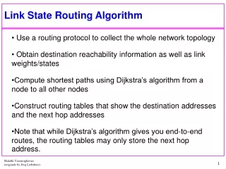
Recap of Previous Lecture • Problems with Distance Vector – Loops • “Bouncing” Effect • Bad news propagates slowly • “Counting to Infinity” • Split Horizon with Poison Reverse • Dijkstra as alternative Shortest Path algorithm to distributed Bellman-Ford Equation • Iteratively grow a shortest path spanning tree from the root outwards • Link-state routing = • Dijkstra shortest path algorithm, + • Reliable flooding of LSPs to all nodes Prof. Rick Han, University of Colorado at Boulder
Link State vs. Distance Vector • Routing update size • LS: small, contain only neighbors’ link costs • DV: potentially long distance vectors (length N for N nodes in network) • Routing update communication overhead • LS: flood to all nodes, overhead is O(N*E), where N is # nodes, and E is # edges or links • In DV, send distance vector only to neighbors Prof. Rick Han, University of Colorado at Boulder
Link State vs. Distance Vector(2) • Convergence speed: • DV: at each iteration, send to neighbor and recalculate • takes awhile to propagate changes to rest of network • Iterations are periodic, hence slow; faster when triggered • LS: faster – don’t need to recalculate LSPs before forwarding • may be key reason that LS beat out DV in intra-domain routing Prof. Rick Han, University of Colorado at Boulder
Link State vs. Distance Vector (3) • Space requirements: • LS maintains entire topology in a link database • DV maintains only neighbor state • If each of N routers has K neighbors, • LS ~ O(N*K) memory requirement • DV ~ O(N*K) also Prof. Rick Han, University of Colorado at Boulder
Link State vs. Distance Vector (4) • Complexity (initializing from scratch) • DV ~ O(N*K*Diameter) • for each of N rows in distance table, find min of (dik+Dkj) over K neighbors, iterate until get info via DV’s of furthest nodes (a diameter away) • If sorted list kept, reduce complexity to O(N*log(K)*Diam.) • LS ~ O(N(N-1)/2)) ~ O(N2) • First iteration, find min cost node from N-1 nodes not in SPT; for 2nd iteration, find min cost node from N-2 nodes not in SPT, … • If a sorted list kept, reduce complexity to O(N*log(N)) • After convergence, new routing updates may only spur partial recalculations for both DV & LS Prof. Rick Han, University of Colorado at Boulder
Link State vs. Distance Vector (5) • Robustness: • Both LS and DV can be completely disabled by a single router advertising false/corrupt LSP or DV • LS can flood false/corrupt LSPs to all routers • DV can advertise false paths/costs to all neighbors • In ARPANET, malfunctioning routers have advertised zero cost, creating a “black hole” • In 1997, a bad router in a small ISP advertised a false cost, became flooded with traffic, disconnecting ISPs from most U.S. backbone providers for ~ 3 hours Prof. Rick Han, University of Colorado at Boulder
Link State vs. Distance Vector (5) • Bottom line: • no clear winner in terms of complexity, space, robustness, … • but LS is favored in the intra-domain Internet due to faster convergence Prof. Rick Han, University of Colorado at Boulder
Link-State Cost Metric • Choice of link cost defines traffic load • Low cost = high probability link belongs to SPT and will attract traffic, which increases cost • Choices for metric: • hop count • queueing delay • Transmission delay • Propagation delay • $$ Prof. Rick Han, University of Colorado at Boulder
Link-State Cost Metric (2) • Static metrics (e.g. hop count or another fixed cost) • Less overhead than dynamic metrics: • flood LSP’s once initially, • Thereafter, flood LSPs only if link fails • Don’t have to deal with staleness • Dynamic metrics can be out of date by the time they arrive at a distant router Prof. Rick Han, University of Colorado at Boulder
Link-State Cost Metric (3) • Dynamic metrics take into account • Changes in link delay (due to congestion) • Variations in link capacity (wireless BW) • Dynamic metrics should: • Avoid oscillations: • low cost attracts traffic => increase cost => less traffic => low cost => increase traffic => increase cost… • Achieve good network utilization • Use link BW efficiently • Limit overhead from flooding LSP’s • Respond quickly, to avoid performing Dijkstra on stale info Prof. Rick Han, University of Colorado at Boulder
Original LS ARPANET Metric • Cost proportional to queue size • Instantaneous queue length as delay estimator • Problems • Did not take into account link speed • Did not take into account propagation delay of a link • Poor indicator of expected delay due to rapid fluctuations • Moves packets toward smallest queue, rather than to destination • Does not achieve good network utilization Prof. Rick Han, University of Colorado at Boulder
New LS ARPANET Metric • Delay = (depart time - arrival time) + transmission time + link propagation delay • (Depart time - arrival time) captures queuing • Transmission time captures link capacity • Link propagation delay captures the physical length of the link • Measurements averaged over 10 seconds • Update sent if difference > threshold, or every 50 seconds • Achieves better network utilization Prof. Rick Han, University of Colorado at Boulder
Problems With New Metric • Works well for light to moderate load • Static values dominate • Oscillates under heavy load • Queuing dominates • Congested link advertising high cost pushes traffic away => some links temporarily underutilized during heavy load – 50% given 2 links between 2 nodes • Range is too wide • 9.6 Kbps highly loaded link can appear 127 times costlier than 56 Kbps lightly loaded link • Can make a 127-hop path look better than 1-hop • Satellite links penalized, though they’d better suit playback video (high BW, non-delay sensitive) Prof. Rick Han, University of Colorado at Boulder
Revised LS ARPANET Metric If a loaded link looks very bad then everyone will move off of it Want some to stay on to balance load and avoid oscillations It is still an OK path for some Use a hop-normalized metric that Has a limited range of values for a given link Doesn’t jump too much between updates for a given link Has a limited range of values across different link types gradual change Prof. Rick Han, University of Colorado at Boulder
Revised LS ARPANET Metric (2) Revised metric is a function of Smoothed bounded link utilization Link type Link utilization Measured link util. is sampled over 10sec period Link utilization = .5*current sample + .5*last average Normalized according to link type Satellite should look good when queuing on other links increases Prof. Rick Han, University of Colorado at Boulder
Routing Metric vs. Link Utilization 225 9.6 satellite 140 New metric (routing units) 90 9.6 terrestrial 75 56 satellite 60 56 terrestrial 30 0 25% 50% 75% 100% Utilization Prof. Rick Han, University of Colorado at Boulder
Observations • Utilization effects • High load never increases cost more than 3*cost of idle link • Cost = f(link utilization) only at moderate to high loads • LSPs flood only if change in Cost exceeds threshold • Link types • Most expensive link is 7 * least expensive link • High-speed satellite link is more attractive than low-speed terrestrial link • Allows routes to be gradually shed from link Prof. Rick Han, University of Colorado at Boulder
Revised LS ARPANET Metric (3) • Better utilization than earlier two metrics • Less oscillation • Allows routes to be gradually shed from link • But is it sufficiently responsive to avoid stale updates? • Can’t propagate updates and react fast enough to short time-scale changes in link cost, so sluggish response is OK • Perlman: “complex….algorithms…bad idea”, “little difference in network capacity between… fixed cost assignment” and dynamic metric Prof. Rick Han, University of Colorado at Boulder
Scalability in Internet Routing • Neither Distance Vector (RIP) nor Link-State (OSPF) scale well to many nodes • DV: slow to propagate and converge • LS: overhead of flooding all nodes to all nodes • DV: 50 million nodes => long distance vectors • Solution: use hierarchy • Group local routers into a domain, can be a subnet on local area or Autonomous System (AS) on wide area • All routers within an AS use an intra-domain routing protocol, e.g. RIP and OSPF • Use another inter-domain routing protocol to route between AS’s Prof. Rick Han, University of Colorado at Boulder
Scalability in Internet Routing (2) Inter-Domain Routing AS 1 AS 2 Border/ Gateway Router Border/ Gateway Router RIP OSPF Intra-Domain Routing Prof. Rick Han, University of Colorado at Boulder
Inter-Domain Routing • Routers within an AS share a common prefix in their IP address, i.e. the top 16 bits are all the same • aggregation of routes • Why Inter-Domain Routing is hard: • 50000 CIDR prefixes to store in each router • Assigning a cost to the AS between two border routers is controlled by owner of each AS • Advertising a cost of 1000 is fast for one AS1, slow for AS2 • Inter-Domain only advertises a “reachable” path across multiple AS’s, not shortest path • Each AS’s owner wants per-route QOS/tariffs • Policy-based routing over performance-based routing Prof. Rick Han, University of Colorado at Boulder
Border Gateway Protocol (BGP) • Similar to Distance Vector, but called “Path” Vector instead • BGP router advertises only reachability info in its vector, not costs/hop counts • E.g. networks 128.96, 192.4.153, and 192.4.3 can be reached from AS2 • BGP router advertises its path to each destination in its vector • Avoids loops Prof. Rick Han, University of Colorado at Boulder
<AS2, R2> <AS2, R1 then R2> <AS2, R3 then R1 then R2> BGP (2) • Each routing update carries the entire path • Loops are detected as follows: • When AS gets route, check if AS already in path • If yes, reject route • If no, add self and (possibly) advertise route further R1 to AS 1 R3 to AS 3 R2 To AS 2 Prof. Rick Han, University of Colorado at Boulder
BGP (3) • How do intra-domain routers learn about routes to other AS’s? • Option 1: Border router injects a default route into intra-domain routing protocol for all addresses not advertised within AS • Option 2: Multiple border routers inject a specific network prefix into intra-domain routing protocol • E.g. “I, BGP 1, have a link to 192.4.54/24 of cost X”, and “I, BGP 2, have a link to 192.4.72/24 of cost Y” Prof. Rick Han, University of Colorado at Boulder
BGP (4) • Perlman: “Although we’re probably stuck with BGP forever, I’ve never been convinced it is the right approach.” • Perlman: “I think the only way to solve the general case of policy-based routing is with a link state protocol plus source-specified routes.” Prof. Rick Han, University of Colorado at Boulder