Download
1 / 27
280 likes | 291 Views
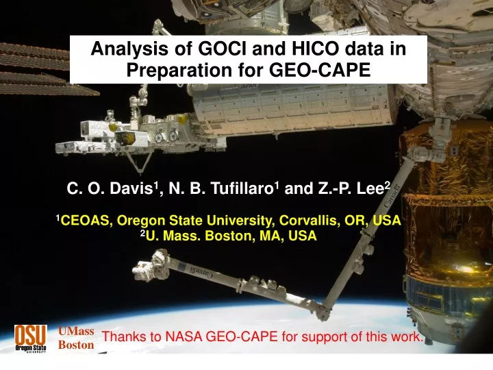
Analysis of GOCI and HICO data in Preparation for GEO-CAPE. C. O. Davis 1 , N. B. Tufillaro 1 and Z.-P. Lee 2 1 CEOAS, Oregon State University, Corvallis, OR, USA 2 U. Mass. Boston, MA, USA. UMass Boston. Thanks to NASA GEO-CAPE for support of this work. Introduction and Outline.

E N D
Analysis of GOCI and HICO data in Preparation for GEO-CAPE C. O. Davis1, N. B. Tufillaro1 and Z.-P. Lee2 1CEOAS, Oregon State University, Corvallis, OR, USA 2U. Mass. Boston, MA, USA UMass Boston Thanks to NASA GEO-CAPE for support of this work.
Introduction and Outline • GEO-CAPE science and requirements • The Hyperspectral Imager for the Coastal Ocean (HICO) • Data Characteristics • Advantage of Hyperspectral • Advantage of 93 m GSD • Geostationary Ocean Color Imager (GOCI) • Data Characteristics • Advantage of hourly data • Combining HICO and GOCI data • GEO-CAPE would like the best of both – is that possible?
The Earth Science Decadal Survey objectives for the GEO Event Imaging mission are to understand and monitor the dynamics of coastal marine ecosystems including their response to land-ocean exchanges, human activity, climate change and episodic events and hazards. GEO-CAPE Ocean objectives have been defined: Quantify the response of marine ecosystems to short-term physical events (e.g., storms and tidal mixing). Assess the importance of high temporal variability in coupled biological-physical coastal-ecosystem models. Monitor biotic and abiotic material in transient surface features (e.g., river plumes and fronts). Detect, track and predict the location of hazardous materials (e.g., oil spills, waste disposal storm events, and harmful algal blooms) GEO-CAPE Oceans Science HICO image: Columbia River Plume, processed to show plume details (N. Tufillaro, C. Davis, OSU)
Why focus on these Requirements? • Because they multiply each other: • Need High SNR (compare threshold to baseline) • Signal is photons collected in the wavelength bin (5 nm or 0.75 nm) for the area imaged (250 m x 250 m = 62,500 m2 vs. 375 x 375 = 140,625 m2 ) over the integration time (1.5 times longer for 375 m). • (22.5 times as much signal per bin for the GEO-CAPE threshold vs. baseline requirements) • Noise is the sum of the instrument noises (small for modern instruments) and the square root of the signal (shot noise or photon noise) nnoise = sqrt(nphoton2 + nCCD2 + nreadout2). (1) • For modern detectors and electronics, nphoton dominates the noise with nphoton2 >> nCCD2 + nreadout2. • But the higher spatial resolution and higher spectral resolution means lower signal per bin and therefore lower SNR so must design instrument to compensate: • Larger telescope, but makes larger instrument and higher costs • longer integration time (from GEO) but slower area coverage rate
Requirement: Hyperspectral Imaging • A hyperspectral imager records a spectrum of the light from each pixel in the scene • Hyperspectral image analysis exploits this extra spectral information • For an open land scene: Total spectrum for a pixel is a weighted sum of the spectra of what is in that pixel Hyperspectral imager Grass Spectral Decomposition for an open land scene + Dry Soil + Leaves + Spectrum for each pixel Camouflage The imager and method of exploitation must be tailored to the scene and the desired products.
Optical Components of a Coastal Scene • Multiple light paths • Scattering due to: • atmosphere • aerosols • water surface • suspended particles • bottom • Absorption due to: • atmosphere • aerosols • suspended particles • dissolved matter • Scattering and absorption are convolved Hyperspectral is needed when you image the bottom (Lee and Carder 2002, Lee et al. 2007), but is it needed for less complex optically deep scenes?
Requirement: High SNR for science needs • Hu, et al. on Ocean Color SNR requirements: • Developed standard radiances for setting ocean SNR requirements • Compared existing systems • Recommendations for future systems (evaluate with GOCI data)
GEO-CAPE requirement 250-375 m at nadir. Requirement: Resolve Coastal Ocean Spatial Scales • Davis et al. on spatial scales: • calculated the lagged distance and semivariance values using “Queen’s move” pixel pairs for airborne Hyperspectral data of Monterey Bay, CA • 100 m GSD ideal for coastal imaging, 300-500 m OK • Will add analysis of HICO 92 m GSD data from a variety of ocean sites
What is the Hyperspectral Imager for the Coastal Ocean (HICO)? • HICO is an experiment to see what we gain by imaging the coastal ocean at higher resolution from space. • The HICO sensor: • first spaceborne imaging spectrometer for coastal oceans • samples coastal regions at <100 m (400 to 900 nm: at 5.7 nm) • high signal-to-noise ratio to resolve the complexity of the coastal ocean • Sponsored as an Innovative Naval Prototype (INP) by the Office of Naval Research: Goal to reduce cost and a greatly shortened schedule. • Start of Project to Sensor Delivery in 16 months • Launched to the ISS September 10, 2009 HICO image of Hong Kong, October 2, 2009. HICO is integrated and flown under the direction of DoD’s Space Test Program
HICO Flight Sensor - Stowed position spectrometer camera lens View port
HICO meets Performance Requirements Parameter Performance Rationale Spectral Range 380 to 960 nm All water-penetrating wavelengths plus Near Infrared for atmospheric correction Spectral Channel Width 5.7 nm Sufficient to resolve spectral features Number of Spectral Channels 102 Derived from Spectral Range and Spectral Channel Width Signal-to-Noise Ratio for water-penetrating wavelengths > 200 to 1 for 5% albedo scene (10 nm spectral binning) Provides adequate Signal to Noise Ratio after atmospheric removal Polarization Sensitivity < 5% (430-1000 nm) Sensor response to be insensitive to polarization of light from scene Ground Sample Distance at Nadir 92 meters Adequate for scale of selected coastal ocean features Scene Size 42 x 192 km Large enough to capture the scale of coastal dynamics Cross-track pointing +45 to -30 deg To increase scene access frequency Scenes per orbit 1 maximum Data volume and transmission constraints
Image location 50 km Radiometric Comparison of HICO to MODIS (Aqua) Nearly coincident HICO and MODIS images of turbid ocean off Shanghai, China demonstrates that HICO is well-calibrated HICO Date: 18 January 2010 Time: 04:40:35 UTC Solar zenith angle: 53 Pixel size: 95 m MODIS (Aqua) Date: 18 January 2010 Time: 05:00:00 UTC Solar zenith angle: 52 Pixel size: 1000 m Top-Of-Atmosphere Spectral Radiance East China Sea off Shanghai R.-R. Li and B-C Gao, NRL
Chlorophyll Comparison of HICO to MODIS (Aqua) Nearly coincident MODIS and HICOTM images of the Yangtze River, China taken on January 18, 2010. Left, MODIS image (0500 GMT) of Chlorophyll-a Concentration (mg/m3) standard product from GSFC. The box indicates the location of the HICO image relative to the MODIS image. Right, HICOTM image (0440 GMT) of Chlorophyll-a Concentration (mg/m3). (R-R Li and B-C Gao, NRL)
Andros Island, Bahamas, Oct 22, 2009 bathymetry absorption RGB image
Microcystis bloom in Lake Erie HICO Image of a massive Microcystis bloom in western Lake Erie, September 3, 2011 as confirmed by spectral analysis.
HICO Summary (HICO Docked on the Space Station) Japanese Exposed Facility HICO • Built and launched in 28 months • Over 5000 scenes so far • One more year of operations • Data from: http://hico.coas.oregonstate.edu
Korean Geostationary Ocean Color Imager (GOCI) • GOCI flying on the Korean COMS satellite: • Launch : June 27, 2010 • First image: July 13, 2010 • GOCI data(Level 1B) and GDPS viewer service : Apr. 20, 2011 • GOCI data(Level 2) and GDPS service : Sep. 2, 2011 • GOCI PI Workshop : Jan. 2012 • http://kosc.kordi.re.kr/index.kosc GOCI has 8 ocean color channels, approximately 1000:1 SNR and images the area around Korea hourly at 500 m GSD.
Analysis of GOCI data in Preparation for GEO-CAPE Curtiss Davis, OSU and Zhongping Lee, U. Mass, Boston Inchon Airport 9/24/2011 • Project initiated September 2011 with 6 objectives: • Evaluate pointing stability • Study radiometric sensitivity • Study coastal dynamics • Study the impact of multiple sampling per day • Study algorithm sensitivities • Characterize sun glint patterns • Results to Date: • HICO and GOCI comparisons • Lake Taihu diurnal cycle GOCI 02:16 GMT HICO 02:28 GMT HICO and GOCI spectra at sample points ------ GOCI HICO ___ Radiance (at-sensor) wavelength (nanometers)
Clear Days With Matches at Han River 2012 01 07 January 2012 02 27 February 2012 03 15 March HICO-GOCI Han River Data Sets
N Relative Bathymetry of Han River Area Mud Flats HICO Image off Korean Peninsula Relative Bathymetry Map Retrieved from HICO Image Shallow Water Approx. 1 meter Depth Deep Water Submerged Mud Flat Water Channel Scene ~ 42 km x 192 km Imaged October 21, 2009 Using 810 nm absorption minimum; Bachmann, et al. Marine Geodesy, 33:53–75, 2010 bathymetry algorithm
Temporal resolution of daily dynamics (GOCI data and numerical simulation) (top) Diurnal pattern of both biomass and PAR (dash lines indicate their daily mean, respectively); (bottom) Diurnal primary production (black line), and the modeled daily total PP using either mean biomass and mean PAR (represented by the red solid line) or using diurnal varying biomass and diurnal varying PAR (represented by the dot black line). (top) Image of color index (Cidx) of Lake Taihu on September 14, 2011 derived from GOCI. Start from top left, clock wise: morning to afternoon. (bottom): Percentage difference relative to 8-image average of lake-wise Cidx.
Are we there Yet? Goals for GEO-CAPE GEO-CAPE ocean imager should have or exceed the combination of the abilities of HICO and GOCI • Hyperspectral Imaging. GEO-CAPE is planned to be a hyperspectral imager from 340-1100 nm. Is 5 nm spectral sampling adequate? Is 0.75 nm for NO2 possible? Is hyperspectral necessary (derivative analysis, phytoplankton functional groups, NO2)? • Finer spatial resolution. Is the GOCI resolution sufficient? Ongoing studies with HICO data. • Sensor Stability and Image Quality. GOCI appears to meet these requirement, but the GOCI telescope does not work for GEO-CAPE • Hourly coverage of US Coastal Waters. Preliminary GOCI data results suggest hourly data required for phytoplankton dynamics and coastal dynamics?