Download
1 / 10
110 likes | 140 Views
Blind State-Space Search. Notes for Ch.11 of Bratko For CSCE 580 Sp03 Marco Valtorta. State-Space Search Formulation of Problem Solving. Initial state a distinguished node in a directed graph Goal state(s) a (set of) distinguished nodes in a directed graph

E N D
Blind State-Space Search Notes for Ch.11 of Bratko For CSCE 580 Sp03 Marco Valtorta
State-Space Search Formulation of Problem Solving • Initial state • a distinguished node in a directed graph • Goal state(s) • a (set of) distinguished nodes in a directed graph • sometimes represented implicitly as a predicate • Possible actions (moves) • edges (arcs) in a directed graph • usually represented by a successor function
State-Space Search Problem Solution • A path in the directed graph representing the problem • shortest • cheapest (least-cost) • Examples (puzzles and practical problems): • block rearrangement (figs.11.1 and 11.2) • traveling salesman • towers of Hanoi • eight puzzle (fig. 11.3) • farmer, wolf, cabbage • eight queens • VLSI placement • other examples: see Ch.3 of Russell and Norvig
Block Rearrangement: Details • state: a list of the three stacks on the table: • e.g., [[c,a,b],[ ],[ ]]---top block is head of list • three goal states: • [[a,b,c],[],[]], [[],[a,b,c],[]], [[],[],[a,b,c]]---a on top • moves (of equal cost; s for successor): • s(Stacks,[Stack1,[Top|Stack2]|OtherStacks]) :- del([Top1|Stack1],Stacks,Stacks1), del(Stack2,Stacks1,OtherStacks). • goal condition: • goal(Situation) :- member([a,b,c],Situation). • initial state is Start in • solve( Start,Solution).
Depth-first Search • To find a solution path, Sol, from a given node N to some goal node, • if N is a goal node, then Sol = [N] • if there is a successor node, N1, of N, such that there is a path Sol1 from N to a goal node, then Sol = [ N | Sol1]. • solve( N,[N]) :- goal( N). • solve( N,[ N|Sol1]) :- s( N,N1), solve( N1,Sol1). • solve is a depth-first program! • solve exploits the depth-first order in which Prolog explores goal trees. • Example: Figure 11.4
Refinement of DFS • Cycle detection • fig11_7.pl (add parentheses for nots!) • depth-limited depth-first search • fig11_8.pl • iterative-deepening depth-first search • ch11_1.pl
Breadth-First Search • To do BFS when given a set of candidate path: • If the head of the first path is a goal node, then this path is a solution, else • Remove the first path from the candidate set and generate the set of one-step extensions of this path, add this set of extensions at the end of the candidate set, and execute BFS on this updated set.
BFS Programs • fig11_10.pl • Basic program • fig11_11.pl • Uses difference lists for open list management
Complexity of Blind Search Procedures • See Table 11.1 • See Ch.3 [Russell and Norvig] • Discusses Dijkstra’s shortest path algorithm also • Dijkstra’s algorithm is optimal among admissible blind unidirectional algorithms, according to the measure “number of node expansions.” • The implementation of Dijkstra’s algorithm that uses heaps is optimal in the decision tree model (Kingston) • IDDFS is, in practice, best, because of the enormous savings in space.
Lower Bound for Dijkstra’s Algorithm • A simple adversary argument shows that any algorithm for shortest paths must examine all edges of a graph (in the worst case): Ω(n+m) lower bound • It is possible to transform (in linear time) sorting to shortest paths, and transform the result back to sorting: Ω(n log n) lower bound in the decision tree model • The implementation of Dijkstra’s algorithm that uses Fibonacci heaps (for the priority queue) achieves the Ω(m + nlogn) lower bound • To improve, either • Go outside the decision tree model (e.g., use radix sorting for the priority queue) • Use an algorithm that cannot generate the sequence of expanded nodes in non-decreasing order from the start node (e.g., use bi-directional search)