Download
1 / 76
770 likes | 1k Views
Chapter 4: Making Statistical Inferences from Samples. 4.1 Introduction 4.2 Basic univariate inferential statistics 4.3 ANOVA test for multi-samples 4.4 Tests of significance of multivariate data 4.5 Non-parametric methods 4.6 Bayesian inferences 4.7 Sampling methods

E N D
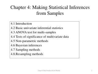
Chapter 4: Making Statistical Inferences from Samples 4.1 Introduction 4.2 Basic univariate inferential statistics 4.3 ANOVA test for multi-samples 4.4Tests of significance of multivariate data 4.5 Non-parametric methods 4.6 Bayesian inferences 4.7 Sampling methods 4.8.Resampling methods Chap 4-Data Analysis Book-Reddy
4.1 Introduction The primary reasons for resorting to sampling as against measuring the whole population is: • to reduce expense • to make quick decisions (say, in case of a production process), • often it is impossible to do otherwise. Random sampling, the most common form of sampling, involves selecting samples from the population in a random manner (the samples should be independent so as to avoid bias- not as simple as it sounds) Such inferences, usually involving descriptive measures such as the mean value or the standard deviation, are called estimators. These are mathematical expressions to be applied to sample data in order to deduce the estimate of the true parameter. Chap 4-Data Analysis Book-Reddy
Fig. 4.13 Overview of various types of parametric hypothesis tests treated in this chapter along with section numbers. The lower set of three sections treat non-parametric tests. • Two types of tests: • Parametric and • Non-parametric Chap 4-Data Analysis Book-Reddy
4.2 Basic Univariate 4.2.1(a) Sampling distribution of the mean Consider a population from which many random samples are taken. What can one say about the distribution of the sample estimators? Let be the population mean and sample mean respectively, be the population std dev and sample std dev Then, regardless of the shape of the population frequency distribution: 4.1 And std dev of the population mean (or SE or standard error of the mean) 4.2 where n is the number of samples selected. Use sample std dev if population std dev is not known Chap 4-Data Analysis Book-Reddy
Fig. 4.1 Illustration of the Central Limit Theorem. The sampling distribution of contrasted with the parent population distribution for three cases with different parent distributions:as sample size increases, the sampling distribution gets closer to a normal distribution (and the standard error of the mean decreases) Chap 4-Data Analysis Book-Reddy
Galton’s Boards (1889) If a ball bounces to the right k times on its way down (and to the left on the remaining pins) it ends up in the kth bin counting from the left. Denoting the number of rows of pins in a bean machine by n, the number of paths to the kth bin on the bottom is given by the binomial coefficient . If the probability of bouncing right on a pin is p (which equals 0.5 on an unbiased machine) the probability that the ball ends up in the kth bin equals is the probability mass function of a binomial distribution. According to the central limit theorem the binomial distribution approximates the normal distribution provided that n, the number of rows of pins in the machine, is large. The machine consists of a vertical board with interleaved rows of pins. Balls are dropped from the top, and bounce left and right as they hit the pins. Eventually, they are collected into one-ball-wide bins at the bottom. The height of ball columns in the bins approximates a bell curve
4.2.1(b) Confidence limits for the mean Instead of the behavior of many samples all taken from one population, what can one say about only one large random sample. This process is called inductive reasoning or arguing backwards from a set of observations to a reasonable hypothesis. However, the benefit provided by having to select only a sample of the population comes at a price: one has to accept some uncertainty in our estimates. Based on a sample taken from a population: • one can deduce intervals bounds of the population mean at a specified confidence level • one can test whether the sample mean differs from the presumed population mean Chap 4-Data Analysis Book-Reddy
4.2.1(b) Confidence limits for the mean The confidence intervalof the population mean = 4.5b This formula is valid for any shape of the population distribution provided, of course, that the sample is large (say, n>30). Half-width of the 95% CL is ( ) : bound of the error of estimation For small samples (n<30), instead of variable z, use student-t variable. Eq.4.5 corresponds to the long-run bounds, i.e., in the long run roughly 95% of the intervals will contain . Prediction of a single x value: Prediction interval of x = 4.6 where tc/2 is the two-tailed critical value at d.f. = n-1 at the desired CL Chap 4-Data Analysis Book-Reddy
Example 4.2.1:Evaluating manufacturer quoted lifetime of light bulbs from sample data A manufacturer claims that the distribution of the lifetimes of his best model has a mean = 16 years and standard deviation = 2 years when the bulbs are lit for 12 hours every day. Suppose that a city official wants to check the claim by purchasing a sample of 36 of these bulbs and subjecting them to tests that determine their lifetimes. • Assuming the manufacturer’s claim to be true, describe the sampling distribution of the mean lifetime of a sample of 36 bulbs. Even though the shape of the distribution is unknown, the Central Limit Theorem suggests that the normal distribution can be used: years. Chap 4-Data Analysis Book-Reddy
Fig. 4.2 Sampling distribution of for a normal distribution N(16, 0.33).Shaded area represents the probability of the mean life of the bulb being < 15 years ii) What is the probability that the sample purchased by the city officials has a mean-lifetime of 15 years or less? The normal distribution N (16, 0.33) is drawn and the darker shaded area to the left of x=15 provides the probability of the city official observing a mean life of 15 years or less. Next, the standard normal statistic is computed as: This probability or p-value can be read off from Table A3 as p( ) = 0.0013. Consequently, the probability that the consumer group will observe a sample mean of 15 or less is only 0.13%. Chap 4-Data Analysis Book-Reddy
(c)If the manufacturer’s claim is correct, compute the ONE TAILED 95% prediction interval of a single bulb from the sample of 36 bulbs. From the t-tables (Table A4), the critical value is tc=1.7 for d.f .=36-1=35 and CL=95% corresponding to the one-tailed distribution. 95% prediction value of x= = = 12.6 years. Chap 4-Data Analysis Book-Reddy
4.2.2 Hypothesis Tests for Single Sample Mean During hypothesis testing the intent is to decide which of two competing claims is true. For example, one wishes to support the hypothesis that women live longer than men. Samples from each of the two populations are taken, and a test, called statistical inferenceis performed to prove (or disprove) this claim. Since there is bound to be some uncertainty associated with such a procedure, one can only be confident of the results to a degree that can be stated as a probability. If this probability value is higher than a pre-selected threshold probability, called significance level of the test, then one would conclude that women do live longer than men; otherwise, one would have to accept that the test was non-conclusive. Chap 4-Data Analysis Book-Reddy
Once a sample is drawn, the following steps are performed: • formulate the hypotheses: the null or status quo, and the alternate (which are complementary) • select a confidence level and estimate the corresponding significance level (say, 0.01 or 0.05) • identify a test statistic (or random variable) that will be used to assess the evidence against the null hypothesis • determine the critical or threshold value of the test statistic from probability tables • compute the test statistic for the problem at hand • rule out the null hypothesis only if the absolute value is greater than the critical statistic , and accept the alternate hypothesis Chap 4-Data Analysis Book-Reddy
Fig. 4.4 Illustration of critical cutoff values between one tailed and two-tailed tests assuming the normal distribution. The shaded areas represent the probability values corresponding to 95% CL or 0.05 significance level or p =0.05. The critical values shown can be determined from Table A3. Be careful that you select the appropriate significance level when a confidence level is stipulated Chap 4-Data Analysis Book-Reddy
Example 4.2.2. Evaluating whether a new type of light bulb has longer life Traditional light bulbs have: mean life = 1200 hours and standard deviation = 3. To compare the life against that of a new type of light bulb Use the classical test and define two hypotheses: • The null hypothesiswhich represents the status quo, i.e., that the new process is no better than the previous one H0 : = 1200 hours, • The research or alternative hypothesis(Ha) is the premise that > 1200 Say, sample size n = 100 and significance or error level of the test is = 0.05. Use one-tailed test (since the new bulb manufacturing process should have a longer life, not just different from that of the traditional process). Chap 4-Data Analysis Book-Reddy
The mean life of the sample of =100 bulbs can be assumed to be normally distributed with mean 1200 and standard error From the standard normal table (Table A3), the one tailed critical z- value is: which leads to =1200+1.64 x 300 /(100)1/2 =1249 • Suppose testing of the 100 tubes yields a value of =1260. As , one would reject the null hypothesis at the 0.05 significance (or error) level. This is akin to jury trials where the null hypothesis is taken to be that the accused is innocent- the burden of proof during hypothesis testing is on the alternate hypothesis. Hence, two types of errors can be distinguished: • Concluding that the null hypothesis is false when in fact it is true is called a Type Ierror, and represents the probability (i.e., the pre-selected significance level) of erroneously rejecting the null hypothesis. This is also called the “false negative” or “false alarm” rate. • The flip side, i.e. concluding that the null hypothesis is true when in fact it is false, is called a Type IIerror and represents the probability of erroneously accepting the alternate hypothesis, also called the “false positive” rate. Chap 4-Data Analysis Book-Reddy
Fig. 4.3 The two kinds of error that occur in a classical test. (a) If H 0 is true, then significance level = probability of erring (rejecting the true hypothesis H0). (b) If Ha is true, then =probability of erring ( judging that the false hypothesis H0 is acceptable). The numerical values correspond to data from Example 4.2.2. False negative False positive Chap 4-Data Analysis Book-Reddy
4.2.3 Two Independent Samples and Paired Difference Tests (a1) Two independent sample test for evaluating the means of two independent random samples from the two populations under consideration whose variances are unknown and unequal (but reasonably close) Test statistic: For large samples, the confidence intervals of the difference in the population means can be determined as: For smaller sample sizes, the z standardized variable is replaced with the student-t variable. The critical values are found from the student t- tables with degrees of freedom d.f.= n1 + n2 -2. 4.7 4.8 Chap 4-Data Analysis Book-Reddy
Fig. 4.5 Conceptual illustration of four characteristic cases that may arise during two-sample testing of medians. The box and whisker plots provide some indication as to the variability in the results of the tests. - Case (a) clearly indicates that the samples are very much different, while the opposite applies to case (d). - However, it is more difficult to draw conclusions from cases (b) and (c), and it is in such cases that statistical tests are useful. (a) (b) (c) (d) Chap 4-Data Analysis Book-Reddy
Example 4.2.3. Verifying savings from home energy conservation measures Certain electric utilities fund contractors to weather strip residences to conserve energy. Suppose an electric utility wishes to determine the cost-effectiveness of their weather-stripping program by comparing the annual electric energy use of 200 similar residences in a given community Samples collected from both types of residences yield: - Control sample: mean = 18,750 ; s1 = 3,200 and n1 = 100. - Weather-stripped sample: mean = 15,150 ; s2 = 2,700 and n2 = 100. The mean difference = =18750 – 15150 = 3,600, i.e., the mean saving in each weather-stripped residence is 19.2% (=3600/18750) However, there is an uncertainty associated with this mean value At the 95% CL, corresponding to a significance level =0.05 for a one-tailed distribution, zc = 1.645 from Table A3, and from eq. 4.8: Chap 4-Data Analysis Book-Reddy
The confidence interval is approximately: =3600 689 = (2,911 and 4,289). These intervals represent the lower and upper values of saved energy at the 95% CL. To conclude, one can state that the savings are positive, i.e., one can be 95% confident that there is an energy benefit in weather-striping the homes. More specifically, the mean saving is 19.2% of the baseline value with an uncertainty of 19.1% (= 689/3600) in the savings at the 95% CL. Thus, the uncertainty in the savings estimate is as large as the estimate itself which casts doubt on the efficacy of the conservation program. This example reflects a realistic concern in that energy savings in homes from energy conservation measures are often difficult to verify accurately. Chap 4-Data Analysis Book-Reddy
4.2.3 Two Independent Samples and Paired Difference Tests (contd.) (a2) “Pooled variances” also used when the samples are small and the variances of both populations are close. Here, instead of using individual standard deviation values s1 and s2, a new quantity called the pooled variance sp is used: with d.f. = n1 + n2-2 - pooled variance is the weighted average of the two sample variances Pooled variance approach is said to result in tighter confidence intervals, and hence its appeal. However, several authors discourage its use Confidence intervals of the difference in the population means is: where Chap 4-Data Analysis Book-Reddy
Example 4.2.4. Comparing energy use of two similar buildings based on utility bills- the wrong way Buildings which are designed according to certain performance standards are eligible for recognition as energy-efficient buildings by federal and certification agencies. A recently completed building (B2) was awarded such an honor. The federal inspector, however, denied the request of another owner of an identical building (B1) close by who claimed that the differences in energy use between both buildings were within statistical error. An energy consultant was hired by the owner to prove that B1 is as energy efficient as B2. He chose to compare the monthly mean utility bills over a year between the two commercial buildings based on the data recorded over the same 12 months and listed in Table 4.1. Chap 4-Data Analysis Book-Reddy
Null hypothesis: mean monthly utility charges for the two buildings are equal . Since the sample sizes are less than 30, the t-statistic has to be used. Pooled variance : and the t-statistic: One-tailed critical value is 1.321 for CL=90 % and d.f.=12+12-2=22: Cannot reject null hypothesis Chap 4-Data Analysis Book-Reddy
There is, however, a problem with the way the energy consultant performed the test. Looking at figure below would lead one not only to suspect that this conclusion is erroneous, but also to observe that the utility bills of the two buildings tend to rise and fall together because of seasonal variations in the climate. Hence the condition that the two samples are independent is violated. It is in such circumstances that a paired test is relevant. Fig. 4.6 Variation of the utility bills for the two buildings B1 and B2 (Example 4.2.5) Chap 4-Data Analysis Book-Reddy
Example 4.2.5.Comparing energy use of two similar buildings based on utility bills- the right way Here, the test is meant to determine whether the monthly mean of the differences in utility charges between both buildings ( ) is zero or not. The null hypothesis is that this is zero, while the alternate hypothesis is that it is different from zero. Thus: = with d.f. = 12-1=11 where the values of 82 and 32 are found from Table 4.1. For = 0.05 with a one-tailed test, from Table A4 critical value t0.05 = 1.796. Because 8.88 >>this critical value, one can safely reject the null hypothesis. In fact, Bldg 1 is less energy efficient than Bldg 2 even at = 0.0005 (or CL = 99.95%), and the owner of B1 does not have a valid case at all! Chap 4-Data Analysis Book-Reddy
4.2.4 Single Sample Tests for Proportions Instances of surveys performed in order to determine fractions or proportions of populations who either have preferences of some sort or have a certain type of equipment- can be interpreted as either a “success” (the customer has gas heat) or a “failure”- a binomial experiment Let p be the population proportion one wishes to estimate from the sample proportion The large sample confidence interval of for the two tailed case at a significance level z 4.13 Chap 4-Data Analysis Book-Reddy
13 131 Chap 4-Data Analysis Book-Reddy
4.2.5 Single (and Two) Sample Tests of Variance Such tests allow one to specify a confidence level for the population variance from a sample Chap 4-Data Analysis Book-Reddy
4.2.6 Tests for Distributions Chap 4-Data Analysis Book-Reddy
Recall the concept of Correlation Coefficient Example 3.4.2. Extension of a spring under different loads: Standard deviations of load and extension are 3.742 and 18.298 respectively, while the correlation coefficient = 0.998. This indicates a very strong positive correlation between the two variables as one should expect. Chap 3-Data Analysis-Reddy
4.2.7 Tests on the Pearson Correlation Coefficient Chap 4-Data Analysis Book-Reddy
Fig. 4.8 Plot depicting 95% confidence bands for population correlation in a bivariate normal population for various sample sizes n. The bold vertical line defines the lower and upper limits of when r = 0.6 from a data set of 10 pairs of observations (from Wonnacutt and Wonnacutt, 1985 by permission of John Wiley and Sons) Chap 4-Data Analysis Book-Reddy
4.3 ANOVA test for multi-samples Fig. 4.9 Conceptual explanation of the basis of an ANOVA test Chap 4-Data Analysis Book-Reddy
error err Chap 4-Data Analysis Book-Reddy
Fig. 4.10 (a) Effect plot. (b) Means plot showing the 95% CL intervals Chap 4-Data Analysis Book-Reddy
A limitation of the ANOVA method is that the null hypothesis is rejected even if one motor bearing is different from the others. In order to pin-point the cause for this rejection, different methods have been developed. One could adopt a paired comparison approach. With 5 sets, 10 paired tests are needed - Tedious - More importantly, sensitivity decreases, i.e., Type I error increases The Tukey method is widely used (applies only when samples are equal) Student t-test is used and approach allows clear visual representation Chap 4-Data Analysis Book-Reddy
Fig. 4.11 Graphical depiction summarizing the ten pairwise comparisons following Tukey’s procedure. Brand 2 is significantly different from Brands 1,3 and 5, and so is Brand 4 from Brand 5 (Example 4.3.2)(bars drawn to correspond to a specified confidence level based on t-tests) Chap 4-Data Analysis Book-Reddy
Fig. 4.12 Two bivariate normal distributions and associated 50% and 90% contours assuming equal standard deviations for both variables. However, the left hand side plots presume the two variables to be uncorrelated, while those on the right have a correlation coefficient of 0.75 which results in elliptical 4.4 Tests of Significance of Multivariate Data (not covered) • Multivariate analysis (also called multifactor analysis) deals with statistical inference and model building as applied to multiple measurements made from one or several samples taken from one or several populations. • They can be used to make inferences about sample means and variances. Rather than treating each measure separately as done in t-tests and single-factor ANOVA, these allow the analyses of multiple measures simultaneously as a system of measurements (results in sounder inferences ) Underlying assumptions of distributions are important: Distortion due to correlated variables Chap 4-Data Analysis Book-Reddy
4.5 Non-Parametric Tests Chap 4-Data Analysis Book-Reddy
4.5.1 Spearman Rank Coefficient Method Chap 4-Data Analysis Book-Reddy
Spearman Rank Correlation Coeff: . where n is the number of paired measurements, and the difference between the ranks for the ith measurement for ranked variables u and v is 0.648 0.648 which suggests that the correlation is not significant. Chap 4-Data Analysis Book-Reddy