Download
1 / 22
250 likes | 489 Views
The turbulent cascade in the solar wind. Luca Sorriso-Valvo LICRYL – IPCF/CNR, Rende, Italy sorriso@fis.unical.it. R. Marino, V. Carbone, R. Bruno, P. Veltri, A. Noullez, B. Bavassano. Turbulence. l. v 0. L. Reynolds Number. Analysis of longitudinal velocity differences.

E N D
The turbulent cascade in the solar wind Luca Sorriso-Valvo LICRYL – IPCF/CNR, Rende, Italy sorriso@fis.unical.it R. Marino, V. Carbone, R. Bruno, P. Veltri, A. Noullez, B. Bavassano
Turbulence l v0 L Reynolds Number Analysis of longitudinal velocity differences
Since dissipation is efficient only at very small scales, the system dissipates energy by transferring it to small scalesNonlinear energy cascade (Richardson picture) Energy cascade Energy injection (e) Integral scale L eddies Non-linear energy transfer (e) Inertial range Energy dissipation (e) Dissipative scale ld
v L Non-linear Re = = n Dissipative Energy injection (e) Integral scale L Non-linear energy transfer (e) Inertial range Energy dissipation (e) Dissipative scale ld Energy balance MHD Navier-Stokes Elsasser fields Enl Ein Eout power-law (observed universal exponent: -5/3)
Phenomenology of fluid turbulence Introducing the energy dissipation rate The characteristic time to realize the cascade (eddy-turnover time) is the lifetime of turbulent eddies Under the Kolmogorov hypothesis (K41) of constant energy transfer rate, the scaling parameter is h = 1/3 This leads to the Kolmogorov scaling law Kolmogorov spectrum
Phenomenological arguments for magnetically dominated MHD turbulence When the flow is dominated by a (large-scale) magnetic field, there is one more characteristic time, the Alfvén time tA, related to the sweeping of Alfvénic fluctuations Since the Alfvén time might be shorter than the eddy-turnover time, nonlinear interactions are reduced and the cascade is realized in a time T A different scaling relation for the pseudo-energies transfer rates Kraichnan spectrum
A puzzle for MHD turbulence Energy cascade needs both z+ and z- fluctuations for the non-linear term to exist. Is the turbulent spectrum compatible with the observed Alfvénic fluctuations ? The energy cascade is due to the nonlinear term of MHD equations Nonlinear interactions occur between fluctuations propagating in opposite direction with respect to the magnetic field. Belcher and Davis, JGR, 1971 Elsasser variables fluctuations z- z+ Observations indicate that one of the Elsasser fluctuations is approximately zero (Alfvénic turbulence), thus the turbulent non-linear Energy cascade should be inhibited.
Evidences of power spectrum in the solar wind attributed to fully developed MHD turbulence Open question about the existence of a MHD turbulent energy cascade Coleman, ApJ, 1968 Bavassano et al., JGR 1982 DYNAMIC ALIGNMENT: Dobrowolny et al. (PRL, 1980) proposed a possible “solution” of the puzzle: if the two Elsasser fields have the same energy transfer rate (same spectral slope), an initial small unbalance at injection scale (meaning quasi-correlated Alfvénic fluctuations) is maintained along a nonlinear cascade toward smaller scales. This is enough to explain the simultaneous observation of a turbulent spectrum and the presence of one single Alfvénic “mode”.
An exact law for incompressible MHD turbulent cascade: Politano & Pouquet From incompressible MHD equations, an exact relation can be derived for the mixed third-order moment assuming stationarity, homogeneity, isotropy (Kolmogorov 4/5) Large-scale inhomogeneities Pressure term (anisotropy) Mixed third-order moment Dissipative term (vanishing in the inertial range) term including the pseudo-energy dissipation rate tensor IF THE YAGLOM RELATION IS VALID, A NONLINEAR ENERGY CASCADE MUST EXIST. THE RELATION IS THE ONLY EXACT AND NONTRIVIALRESULT IN TURBULENCE Politano & Pouquet, PRE 1998 Politano, Pouquet, Carbone,EPL 1998 Sorriso-Valvo et al, PRL 2007
Numerical evidences From 2-dimensional numerical simulation of MHD equations (1024X1024) A snapshot of the current j from the simulation in the statistically steady state Sorriso-Valvo et al, Phys. of Plasmas 2002
Ulysses data 1996: results Low solar activity (1994-1996) High latitude (q > 35°) 8 minutes averages of velocity, magnetic field and density are used to build the Elsasser fields Z± Running windows of 10 days (2000 data points each) have been used to avoid radial distance and latitudinal variations, as well as non-stationariety effects.
1. Observation of inertial range scaling The Politano & Pouquet relation is satisfied in several Ulysses samples (polar, fast wind high Alfvénic correlations!) Although the data may be affected by inhomogeneity, local anisotropy and compressible effects, the observed P&P scaling law is robust in most periods of Ulysses dataset. The first REAL evidence that (low frequency) solar wind can be described in the framework of MHD turbulence Sorriso-Valvo et al., PRL (2007)
2. The energy transfer rates The estimated values of energy transfer rates are about 100J/Kg sec. For comparison, energy transfer rates per unit mass in usual fluid flows are 1 50 J/Kg s
3. The inertial range of SW turbulence In literature: up to 6-12 hours. Our data: up to 1-2 days. What is the actual extent of the inertial range in SW? Radial velocity and magnetic field spectra for one sample of wind with Yaglom scaling Ev The velocity spectrum extends to large scales, while magnetic spectral break is often (but not always) observed around a few hours. f-5/3 EB Velocity inertial range can locally extend up to 1-2 days! Seen from Yaglom law and from spectral properties. 1day 1h
4. MHD or Navier-Stokes? The role of magnetic field Velocity contribution to energy transport It is possible to separate the contributions to the energy cascade: terms advected by velocity and terms advected by magnetic field. Magnetic contribution to energy transport In this example, Yaglom scaling is dominated by the magnetic field at small scales (from 10 mins to 3h), but at large scale only the velocity advects energy Total energy transport Separation of scales around the Alfvén time
3.-4. Different behaviour in different samples SMALL SCALES (< hours): Magnetic filed dominates or equilibrium: MHD cascade LARGE SCALES (> hours): Velocity dominates (Navier-Stokes cascade), or non- negligible magnetic field contribution (MHD cascade) NON UNIVERSALITY OF SOLAR WIND TURBULENCE!
5. Compressive turbulence in solar wind: phenomenological scaling law Low-amplitude density fluctuations could play a role in the scaling law Energy-transfer rates per unit volume in compressible MHD Introducing phenomenological variables, dimensionally including density Density-weighted Elsasser variables: what scaling law for third-order mixed moment? Kowal & Lazarian, ApJ 2007, Kritsuk et al., ApJ 2007, Carbone et al., PRL 2009
5. Compressive turbulence in solar wind: observation from data Phenomenological compressible P&P enhanced scaling is observed, even in samples where the incompressible law is not verified.
6. Solar wind heating Is the measured turbulent energy flux enough to explain the observed non-adiabatic expansion of the solar wind? Solar wind models Adiabatic expansion, temperature should decrease with helioscentric distance Spacecraft measurements Temperature decay is slower than expected from adiabatic expansion Estimate of the heating rate needed for the solar wind: models for turbulence Vasquez et al., JGR 2007
Compressive and incompressive dissipation rates, compared with model wind heating (2 temperatures) estimated energy transfer rate: compressible case estimated energy transfer rate: incompressible cascade energy transfer rate required for the observed T
7. The role of cross-helicity Cross-helicity plays a relevant role in the MHD turbulent cascade in solar wind. Slow: both modes slow Fast: only one mode fast Fast streams (high cross-helicity) have a weak turbulent cascade on only one mode. Slow streams, in which the two modes coexist and can exchange energy more rapidly, the energy cascade is more efficient (giving larger transfer rates) and is observable on both modes. This observation reinforces the scenario proposed by Dobrowolny et al. suggesting that MHD cascade is favoured in low cross-helicity samples.
Conclusions The MHD cascade exists in the solar wind. First measurements of energy dissipation rate (statistical analysis in progress). The extent of the inertial range is larger than previously estimated. The role of magnetic field is relevant (but not always) for the cascade, especially at small scales. However, no universal phenomenology is observed (work in progress). Density fluctuations, despite their low-amplitude, enhance the turbulent cascade (more theoretical results are needed). Heating of solar wind could be entirely due to the compressible turbulent cascade. Cross-helicity plays an important role in the scaling: Alfvénic fluctuations inhibit the cascade, in the spirit of dynamic alignment (work in progress). The turbulent cascade was observed in Ulysses solar wind data through the Politano & Poquet law, providing several results: