Statistical Inference

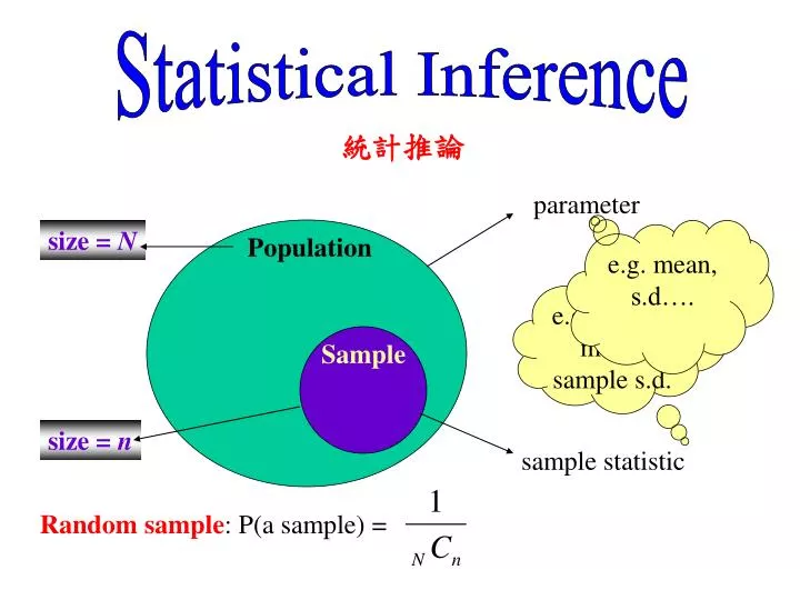
Population Sample Statistical Inference 統計推論 parameter size = N e.g. mean, s.d…. e.g. sample mean, sample s.d. size = n sample statistic Random sample: P(a sample) =

Sample Mean Distribution  and  are fixed, but and s are random variables, So what’s the distribution of the sample mean ?

The mean (i.e. expectation) and the variance of and  can be found easily. But we are not satisfied with only TWO single information, we want to know ALL the situation of i.e. The distribution of

If the distribution of X is normal, the distribution of is also normal, since is the linear combination of Xi. BUT, how about if X is NOT normally distributed?

Central Limit Theorem Although X ~ ? approximately, we still have provided that n is sufficiently large. In practice, n > 30. Great!

E.g. 5 Light bulbs,  = 1800 hrs,  = 200 hrs. Find the prob. that a random sample of 100 bulbs will have average life > 1825 hrs We don’t know what’s the distribution of bulbs’ life!! But, by CLT, we know the sample mean’s distribution!! ~N(1800,400) Thus, = 0.1056

E.g. 7 A driver is allowed to work max. 10 hrs per day. Journey time per delivery:  = 30 min.,  = 8 min. How many deliveries so as to less than 1/1000 chance of exceeding 10 hrs. =30n =n82 Var(X) = nVar(Xi) X~N(30n,64n) By CLT, By question, By table, P(X > 600)  0.001 P(z>3.09) = 0.001

To ensure the chance < 0.001, we can take:  4.08 or 4.9 (rejected) n 16 Hence we should schedule 16 or less deliveries per day.

E.g. 10 A die is cast sixty times. Estimate the probability that the total number of points is less than or equal to 200. Let X = total points = 3.5 E(X) = 603.5 = 210 By CLT, Var(X) = 6035/12 = 175 X ~ N(210,175) = 0.236 P(X 200) =

Statistical Inference