Download
1 / 40
400 likes | 562 Views
Statistical inference. Take a random sample of n independent observations from a population. Calculate the mean of these n sample values. This is know as the sample mean . Repeat the procedure until you have taken all possible samples of size n , calculating the sample mean of each.

E N D
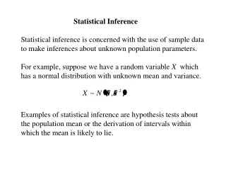
Take a random sample of n independent observations from a population. Calculate the mean of these n sample values. This is know as the sample mean. Repeat the procedure until you have taken all possible samples of size n, calculating the sample mean of each. Form a distribution of all the sample means. The distribution that would be formed is called the sampling distribution of means. Distribution of the sample mean In many cases we need to infer information about a population based on the values obtained from random samples of the population. Consider the following procedure:
Central limit theorem This theorem holds when the population of X is discrete or continuous!! Read Example 9.15, pp.442-443 Do Exercise 9C, pp.443-444
Unbiased estimates of population parameters Suppose that you do not know the value of a particular population parameter of a distribution. It seems sensible to take a random sample from the distribution and use it in some way to make estimates of unknown parameters. The estimate is unbiased if the average (or expectation) of a large number of values taken in the same way is the true value of the parameter. Point estimates Read Example 9.17, p.448
Is the distribution of the population normal or not? Is the variance of the population known? Is the sample size large or small? Unbiased estimates of population parameters Interval estimates Another way of using a sample value to estimate an unknown population parameter is to construct an interval, known as a confidence interval. This is an interval that has a specified probability of including the parameter. Three questions
Confidence interval for µ(normal population, known population variance, any sample size) The goal is to calculate the end-values of a 95% confidence interval. We can adapt this approach for other levels of confidence. Read Example 9.19, pp.451-452
Confidence interval for µ(normal population, known population variance, any sample size) This computer simulation shows 100 confidence intervals constructed at the 95% level. On average 5% do not include µ. In other words, on average, 95% of the intervals constructed will include the true population mean. Critical z-values in confidence intervals The z-value in the confidence interval is known as the critical value.
Read Examples 9.20 – 9.22, pp.454-457 Confidence interval for µ(non-normal population, known population variance, large sample size) Note • for a given sample size, the greater the level of confidence, the wider the confidence interval; • for a given confidence level, the smaller the interval width, the larger the sample size required; • for a given interval width, the greater the level of confidence, the larger the sample size required.
Confidence interval for µ(any population, unknown population variance, large sample size) Read Examples 9.23 & 9.24, pp.458-459 Do Exercise 9e, pp.460-461
Confidence interval for µ(normal population, unknown population variance, small sample size) For small samples:
Confidence interval for µ(normal population, unknown population variance, small sample size) The t-distribution
Read Examples 9.26 & 9.27, pp.466-468 Do Exercise 9f, p.468 Confidence interval for µ(normal population, unknown population variance, small sample size)
Confidence intervals for µ Read Examples 9.30, pp. 474-475 Read Examples 9.32 & 9.33, pp. 476-478 Do Exercise 9h, Q1-Q4, Q7, Q10-Q12, Q15, Q17-Q21, pp.478-481
Hypothesis testing- example A machine fills ice-packs with liquid. The volume of liquid follows a normal distribution with mean 524 ml and standard deviation 3 ml. The machine breaks down and is repaired. It is suspected the machine now overfills each pack, so a sample of 50 packs is inspected. The sample mean is found to be 524.9 ml. Is the machine over-dispensing? Is the sample mean high enough to say that the mean volume of all packs has increased? A hypothesis (or significance) test enables a decision to be made on this question. The test is now carried out.
Hypothesis testing- example The result of the test depends on the location in the sampling distribution of the test value524.9 ml. If it is close to 524 then it is likely to have come from a distribution with mean 524 ml and there would not be enough evidence to say the mean volume has increased. If it is far away from 524 (i.e. in the upper tail of the distribution) then it is unlikely to have come from a distribution with mean 524 ml and the mean is likely to be higher that 524 ml.
Hypothesis testing- example Conclusion: There is evidence, at the 5% level, that the mean volume of liquid being dispensed by the machine has increased.
Critical z-values and rejection criteria Example: At the 1% level One-tailed tests Two-tailed tests
Testing the mean, µ, of a population(normal population, known variance, any sample size) Read Examples 11.1 & 11.2, pp.514-517
Testing the mean, µ, of a population(non-normal population, known variance, large sample size) Read Examples 11.3, pp.517-518
Read Examples 11.4, pp.519-520 Testing the mean, µ, of a population(any population, unknown variance, large sample size) Do Exercise 11A, Q1-Q6, Q8-Q10, Q13, pp.522-523
Testing the mean, µ, of a population(normal population, unknown variance, small sample size) Read Examples 11.6 &11.7, pp.524-526 Do Exercise 11b, pp.527-528
Read Examples 11.11 - 11.15, pp.536-542 Do Exercise 11d, Sections A & B, pp.543-546
Paired samples It is widely thought that people’s reaction times are shorter in the morning and increase as the day goes on. A light is programmed to flash at random intervals and the experimental subject has to press a buzzer as soon as possible and the delay is recorded. Experiment 1: Two random samples of 40 students are selected from the school register. One of these samples, chosen at random, uses the apparatus during the first period of the day, while the second sample uses the apparatus during the last period of the day. The means of the two samples are compared. Experiment 2: A random sample of 40 students is selected from the school register. Each student is tested in the first period of the day, and again in the last period. The difference in reaction times between the two periods for each student is calculated. The mean difference is compared with zero. Experiment 1 requires a standard two-sample comparison of means, assuming a common variance. There is nothing wrong with this procedure but we could be misled. Firstly, suppose that all the bookworms were in the first sample and all the athletes in the second- we might conclude that reaction times decrease over the course of the day! More subtly, the variations between the students may be much greater than any changes in individual students over the time of day; these changes may pass unnoticed. In Experiment 2 the variability between the students plays no part. All that matters is the variability of the changes within each student’s readings. The problems with Experiment 1 have vanished! Experiment 2 is a paired-sample test.
The paired-sample comparison of means We have created a single sample situation, so previous methods now apply!
Distinguishing between thepaired-sample and two-sample cases • If the two samples are of unequal size then they are not paired. • Two samples of equal size are paired only if we can be certain that each observation from the second sample is associated with a corresponding observation from the first sample.
A significance test for the product-moment correlation coefficient Read Examples 13.1, pp.603-604 Do Exercise 13a, p.604