Download
1 / 21
210 likes | 214 Views
This article explores the concepts of fluid boundaries, discontinuities, and shocks, and the equations that govern their behavior. It covers topics such as Rankine-Hugoniot conditions, bow shock geometry, and different types of shocks. The text language is English.

E N D
Boundaries, shocks and discontinuities • Fluid boundaries • General jump conditions • Rankine-Hugoniot conditions • Set of equations for jumps at a boundary • Discontinuities • Shock types • Bow shock geometry
Fluid boundaries Equilibria between plasmas with different properties give rise to the evolution of boundaries, which take the form of narrow (gyrokinetic scales) layers called discontinuities. Conveniently, one starts from ideal plasmas (without dissipation) on either side. The transition from one side to the other requires some disspation, which is concentrated in the layer itself but vanishes outside. MHD (with ideal Ohm‘s law and no space charges) in conservation form reads:
Definitions, normal and jumps Changes occur perpendicular to the discontinuity, parallel the plasma is uniform. The normal vector, n, to the surface S(x) is defined as: Any closed line integral (along a rectangular box tangential to the surface and crossing S from medium 1 to 2 and back) of a quantity X reduces to Since an integral over a conservation law vanishes, the gradient operation can be replaced by Transform to a frame moving with the discontinuity at local speed, U. Because of Galilean invariance, the time derivative becomes:
Discontinuities and shocks Continuity of the mass flux and magnetic flux: Bn = B1n = B2n Gn = 1(V1n - U) = 2(V2n - U) U is the speed of surface in the normal direction; B magnetic field vector; V the flow velocity. Mach number,M = V/C. Here C is the wave phase speed. Contact discontinuity (CD) Index 1 upstream and 2 downstream; B does not change across the surface of the CD, but 1 2 and T1 T2 . Shock: G 0 Discontinuity: G = 0
Rankine-Hugoniot conditions I In the comoving frame (v' = v - U) the discontinuity (D) is stationary so that the time derivative can be dropped. We skip the prime and consider the situation in a frame where D is at rest. We assume an isotropic pressure, P=p1. Conservation laws transform into the jump conditions across D, reading: An additional equation expresses conservation of total energy across the D, whereby w denotes the specific internal energy in the plasma, w=cvT.
Rankine-Hugoniot conditions II The normal component of the magnetic field is continuous: The mass flux across D is a constant: Using these two relations and splitting B and v into their normal (index n) and tangential (index t) components gives three remaining jump conditions: stress balance tangential electric field pressure balance These equations contain all basic information about any D in ideal MHD.
Mass-flux classification of D‘s Introduce the average of X across a D by the mean value: New variables: Specific volume, V = (nm)-1 and constant normal mass flux, F = nmn.After tedious algebra (left as a hard exercise) the determinant for the system of RHC can be written as a seventh-order equation in F, reading: Tangential, contact D Shocks Rotational D
Contact and tangential discontinuity CD and TD are characterized by a zero normal mass flow, and thus n= 0. Bn 0 -> Contact D Since in a CT the thermal pressure remains constant, any change in density must be compensated by a change in temperature. However, a temperature jump is quickly ironed out by electron heat conduction -> CD do not persist long. Bn= 0 -> Tangential D
Schematic parameter changes across a TD 1 2 Total pressure is constant. TD‘s are often observed in the solar wind.
Rotational discontinuity (RD) RDs are characterized by a finite normal mass flow, but a continuous n. Because of the continuity of F and n, there can be no jump in density. Since Bn and n are constant, the tangential components must rotate together! Constant normal n leads naturally to a constant vAn. Thus the so-called Walen relation holds:
Schematic parameter changes across a RD The RD jump conditions imply the Walén relation: 8.42 1 2 At a RD the jump in tangential flow velocity is exactly equal to the jump in tangential Alfvén velocity. RD‘s occur frequently in the fast solar wind.
Entropy changes at discontinuities Instead of the energy conservation equation one may use the entropy equation, which can without dissipation be written as: For an ideal isotropic gas we have (with gas constant R0 and polytropic index =5/3) the entropy change: In a steady state incompressible medium: Or written as a jump condition: • Discontinuity (D) with [n] = 0 conserves entropy • D in compressible medium with [n] 0 leads to increase of entropy
Shocks This third type of D is characterised by a non-vanishing normal mass flux, F = nmn 0. F is a solution of the bi-quadratic equation: Shock solutions are obtained if the specific volume V = (nm)-1 jumps, and since F2 must be positive, the following inequality holds: This condition is easily satisfied if the right ratio is negative, hence when pressure and specific volume vary oppositely across the D; --> shock
Machnumbers We may multiply the previous equation for the normal mass flux, F = nmvn, by 2 = <(nm)-1>2, and introduce the following two speeds: Effective Alfvén speeds: UA2 = B2/0 ; UAn2 = Bn2 /0 Effective sound speed: CS2 = - ( p / ) 2 Effective shock speed: U= F In terms of these speeds the shock „dispersion equation“ can be written as: U4 - U2(UA2+CS2) + CS2UAn2 = 0 This yields the fast and slow magnetoacoustic velocities, UF and US, as possible solutions. The corresponding Machnumbers are: MF,S = U/UF,S.
Coplanarity Knowing that for the shock n 0 and [n ] 0, we can eliminate [t ] from the RHCs and obtain: Hence the cross product of the left with the right hand side must vanish: When resolving these brackets one obtains the condition: The resulting coplanarity theorem implies that the magnetic field across the shock has a 2-D geometry: upstream and dowstream tangential fields are parallel to each other and coplanar with the shock normal n.
Shock jump conditions We use for the sake of simplicity the internal energy for a monoatomic gas under adiabatic conditions: w=p/(nm( -1)). With this the energy conservation can be brought in a form using jumps and averages: Exploiting the coplanarity condition, we can write the tangential components in scalar form as follows: These equations form a closed set for the jumps in shocks (general RHCs).
Fast and slow shocks By eliminating the jump in the normal velocity [vn] one can obtain a relation between the jumps in the thermal and tangential magnetic pressure (where the quantity H is defined below): Since always [p] > 0 for shocks, because the disturbed plasma is compressed and heated, one can distinguish between two shock types: Fast shocks with increasing magnetic pressure, Bt2 > 0 , satisfying vn > ( -1)H and MF > 1 Slow shocks with decreasing magnetic pressure, Bt2 < 0 , satisfying vn < ( -1)H and MS > 1
Schematic parameter changes across a fast shock 1 2 In a fast shock the magnetic field increases. It is tilted toward the surface and bends away from the normal. Fast shocks may evolve from fast mode waves.
Schematic parameter changes across a slow shock 1 2 In a slow shock the magnetic field decreases. It is tilted away from the surface and bends toward the normal. Slow shocks may evolve from slow mode waves.
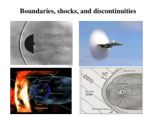
Bow shock The most famous and mostly researched shock is the bow shock standing in front of the Earth as result of the interaction of the magnetosphere with the supersonic solar wind, with a high Machnumber, MF 8. Solar wind density and field jump by about a factor of 4 into the magnetosheath.