Download
1 / 38
380 likes | 401 Views
Learn about various data types, attributes, and statistical analysis techniques. Explore data objects, attribute types, and basic statistical descriptions. Understand data mining concepts and techniques for effective analysis.

E N D
Mengenal dan memahami data • Objek data dan macam-macam atribut • Statistik diskriptif data • Visualisasi data • Mengukur kesamaan dan ketidaksamaan data
Types of Data Sets • Record • Relational records • Data matrix, e.g., numerical matrix • Document data: text documents: term-frequency vector • Transaction data • Graph and network • World Wide Web • Social or information networks • Ordered • Video data: sequence of images • Temporal data: time-series • Spatial, image and multimedia: • Spatial data: maps • Image data: • Video data:
Data Objects • Data object menyatakan suatu entitas • Contoh: • Database penjualan: customers, barang-barang yang dijual, penjualan • Database medis: pasien, perawatan • Database universitas: mahasiswa, professor, perkuliahan • Data objects dijelaskan dengan attribut-atribut. • Baris-baris Database -> data objects; • Kolom-kolom ->attribut-atribut.
Atribut • Attribut ( dimensi, fitur, variabel): menyatakan karakteristik atau fitur dari data objek • Misal., ID_pelanggan, nama, alama • Tipe-tipe: • Nominal • Ordina • Biner • Numerik: • Interval-scaled • Ratio-scaled
Attribute Types • Nominal: kategori, keadaan, atau “nama suatu hal” • Warna rambut • Status , kode pos, dll, NRP dll • Binary :Atribut Nominal dengan hanya 2 keadaan (0 dan 1) • Symmetric binary: keduanya sama penting • Misal: jenis kelamin, • Asymmetric binary: keduanya tidak sama penting. • Misal : medical test (positive atau negative) • Dinyatakan dengan 1 untuk menyatakan hal yang lebih penting ( positif HIV) • Ordinal • Memiliki arti secara berurutan, (ranking) tetapi tidak dinyatakan dengan besaran angka atau nilai. • Size = {small, medium, large}, kelas, pangkat
Atribut Numerik • Kuantitas (integer atau nilai real) • Interval • Diukur pada skala dengan unit satuan yang sama • Nilai memiliki urutan • tanggal kalender • No true zero-point • Ratio • Inherent zero-point • Contoh:Panjang, berat badan, dll • Bisa mengatakan perkalian dari nilai objek data yang lain • Misal : panjang jalan A adalah 2 kali dari panjang jalan B
Atribut Discrete dan kontinu • Atribut Diskrit • Terhingga, dapat dihitung walaupun itu tak terhingga • Kode pos, kata dalam sekumpulan dokumen • Kadang dinyatakan dengan variabel integer • Catatan Atribut Binary: kasus khusus atribut diskrit • Atribut Kontinu • Memilki nilai real • E.g., temperature, tinggi, berat • Atribut kontinu dinyatakn dengan floating-point variables
Basic Statistical Descriptions of Data • Tujuan • Untuk memahami data: central tendency, variasi dan sebaran • Karakteristik Sebaran data • median, max, min, quantiles, outliers, variance, dll.
Mengukur Central Tendency • Mean (algebraic measure) (sample vs. population): Note: n jumlah sample dan N nilai populasi. • Mean/rata-rata: • Trimmed mean: • Median: • Estimated by interpolation (for grouped data): • Mode • Value that occurs most frequently in the data • Unimodal, bimodal, trimodal • Empirical formula: Median interval
Data Mining: Concepts and Techniques Symmetric vs. Skewed Data • Median, mean and mode of symmetric, positively and negatively skewed data symmetric positively skewed negatively skewed
Mengukur sebaran Data • Quartiles, outliers and boxplots • Quartiles: Q1 (25th percentile), Q3 (75th percentile) • Inter-quartile range: IQR = Q3 –Q1 • Five number summary: min, Q1, median,Q3, max • Outlier: biasanya lebih tinggi atau lebih rendah dari 1.5 x IQR • Variansi dan standar deviasi (sample:s, population: σ) • Variance: (algebraic, scalable computation) • Standard deviation s (atau σ) akar kuadrat daro variance s2 ( atau σ2 )
Boxplot Analysis • Lima nilai dari sebaran data • Minimum, Q1, Median, Q3, Maximum • Boxplot • Data dinyatakan dengan box • Ujung dari box kuartil pertama dan ketiga, tinggi kotak adalah IQR • Median ditandai garis dalam box • Outliers: diplot sendiri diluar
Sifat-sifat kurva Distribusi Normal • Kurva norma • dari μ–σ to μ+σ: berisi 68% pengukukuran (μ: mean, σ: standar deviasi) • Dari μ–2σ to μ+2σ: berisi 95% pengukuran • Dari μ–3σ to μ+3σ: berisi 99.7% pengukuran
Histogram Analysis • Histogram: grafik menampilkan tabulasi dari frekwensi data
Histograms Often Tell More than Boxplots • Dua histogram menunjukkan boxplot yang sama • Nilai yang sama: min, Q1, median, Q3, max • Tetapi distribusi datanya berbeda
Scatter plot • Melihat data bivariate data untuk melihat cluster dan outlier data, etc • Setiap data menunjukkan pasangan koordinat dari suatu data
Positively and Negatively Correlated Data • Kiri atas korelasi positif • Kanan atas korelasi negatif
Data Visualization • Why data visualization? • Gain insight into an information space by mapping data onto graphical primitives • Provide qualitative overview of large data sets • Search for patterns, trends, structure, irregularities, relationships among data • Help find interesting regions and suitable parameters for further quantitative analysis
Geometric Projection Visualization Techniques • Visualization of geometric transformations and projections of the data • Methods • Scatterplot and scatterplot matrices
Scatterplot Matrices Matrix of scatterplots (x-y-diagrams) of the k-dim. data [total of (k2/2-k) scatterplots] Used byermission of M. Ward, Worcester PolytechnicInstitute
Similarity and Dissimilarity • Similarity • Mengukur secara Numerik bagaimana kesamaan dua objek data • Tinggi nilainya bila benda yang lebih mirip • Range [0,1] • Dissimilarity (e.g., distance/jarak) • Ukuran numerik dari perbedaan dua objek • Sangat rendah bila benda yang lebih mirip • Minimum dissimilarity i0
Data Matrix and Dissimilarity Matrix • Data matrix • n titik data dengan p dimensi • Two modes • Dissimilarity matrix • n titik data yang didata adalah distance/jarak • Matrik segitiga • Single mode
Proximity Measure for Nominal Attributes • Misal terdapat 2 atau lebih nilai, misal., red, yellow, blue, green (generalisasi dari atribut binary) • Metode Simple matching • m: # yang sesuai, p: total # variabel
Proximity Measure for Binary Attributes Object j • A contingency table for binary data • Distance measure for symmetric binary variables: • Distance measure for asymmetric binary variables: • Jaccard coefficient (similarity measure for asymmetric binary variables): Object i • Note: Jaccard coefficient is the same as “coherence”:
Dissimilarity between Binary Variables • Example • Gender is a symmetric attribute • The remaining attributes are asymmetric binary • Let the values Y and P be 1, and the value N 0
Standardizing Numeric Data • Z-score: • X: raw score to be standardized, μ: mean of the population, σ: standard deviation • the distance between the raw score and the population mean in units of the standard deviation • negative when the raw score is below the mean, “+” when above • An alternative way: Calculate the mean absolute deviation where • standardized measure (z-score): • Using mean absolute deviation is more robust than using standard deviation
Example: Data Matrix and Dissimilarity Matrix Data Matrix Dissimilarity Matrix (with Euclidean Distance)
Distance on Numeric Data: Minkowski Distance • Minkowski distance: A popular distance measure where i = (xi1, xi2, …, xip) and j = (xj1, xj2, …, xjp) are two p-dimensional data objects, and h is the order (the distance so defined is also called L-h norm) • Properties • d(i, j) > 0 if i ≠ j, and d(i, i) = 0 (Positive definiteness) • d(i, j) = d(j, i)(Symmetry) • d(i, j) d(i, k) + d(k, j)(Triangle Inequality)
Special Cases of Minkowski Distance • h = 1: Manhattan (city block, L1 norm) distance • E.g., the Hamming distance: the number of bits that are different between two binary vectors • h = 2: (L2 norm) Euclidean distance • h . “supremum” (Lmax norm, Lnorm) distance. • This is the maximum difference between any component (attribute) of the vectors
Example: Minkowski Distance Dissimilarity Matrices Manhattan (L1) Euclidean (L2) Supremum
Ordinal Variables • An ordinal variable can be discrete or continuous • Order is important, e.g., rank • Can be treated like interval-scaled • replace xif by their rank • map the range of each variable onto [0, 1] by replacing i-th object in the f-th variable by • compute the dissimilarity using methods for interval-scaled variables
Attributes of Mixed Type • A database may contain all attribute types • Nominal, symmetric binary, asymmetric binary, numeric, ordinal • One may use a weighted formula to combine their effects • f is binary or nominal: dij(f) = 0 if xif = xjf , or dij(f) = 1 otherwise • f is numeric: use the normalized distance • f is ordinal • Compute ranks rif and • Treat zif as interval-scaled
Cosine Similarity • A document can be represented by thousands of attributes, each recording the frequency of a particular word (such as keywords) or phrase in the document. • Other vector objects: gene features in micro-arrays, … • Applications: information retrieval, biologic taxonomy, gene feature mapping, ... • Cosine measure: If d1 and d2 are two vectors (e.g., term-frequency vectors), then cos(d1, d2) = (d1d2) /||d1|| ||d2|| , where indicates vector dot product, ||d||: the length of vector d
Example: Cosine Similarity • cos(d1, d2) = (d1d2) /||d1|| ||d2|| , where indicates vector dot product, ||d|: the length of vector d • Ex: Find the similarity between documents 1 and 2. d1= (5, 0, 3, 0, 2, 0, 0, 2, 0, 0) d2 = (3, 0, 2, 0, 1, 1, 0, 1, 0, 1) d1d2 = 5*3+0*0+3*2+0*0+2*1+0*1+0*1+2*1+0*0+0*1 = 25 ||d1||= (5*5+0*0+3*3+0*0+2*2+0*0+0*0+2*2+0*0+0*0)0.5=(42)0.5 = 6.481 ||d2||= (3*3+0*0+2*2+0*0+1*1+1*1+0*0+1*1+0*0+1*1)0.5=(17)0.5 = 4.12 cos(d1, d2 ) = 0.94
KL Divergence: Comparing Two Probability Distributions • The Kullback-Leibler (KL) divergence: Measure the difference between two probability distributions over the same variable x • From information theory, closely related to relative entropy, information divergence, and information for discrimination • DKL(p(x)||q(x)): divergence of q(x) from p(x), measuring the information lost when q(x) is used to approximate p(x) • Discrete form: • The KL divergence measures the expected number of extra bits required to code samples from p(x) (“true” distribution) when using a code based on q(x), which represents a theory, model, description, or approximation of p(x) • Its continuous form: • The KL divergence: not a distance measure, not a metric: asymmetric, not satisfy triangular inequality
How to Compute the KL Divergence? • Base on the formula, DKL(P,Q) ≥ 0 and DKL(P || Q) = 0 if and only if P = Q. • How about when p = 0 or q = 0? • limp→0p log p = 0 • when p != 0 but q = 0, DKL(p || q) is defined as ∞, i.e., if one event e is possible (i.e., p(e) > 0), and the other predicts it is absolutely impossible (i.e., q(e) = 0), then the two distributions are absolutely different • However, in practice, P and Q are derived from frequency distributions, not counting the possibility of unseen events. Thus smoothing is needed • Example: P : (a : 3/5, b : 1/5, c : 1/5). Q : (a : 5/9, b : 3/9, d : 1/9) • need to introduce a small constant ϵ, e.g., ϵ = 10−3 • The sample set observed in P, SP = {a, b, c}, SQ = {a, b, d}, SU = {a, b, c, d} • Smoothing, add missing symbols to each distribution, with probability ϵ • P′ : (a : 3/5 − ϵ/3, b : 1/5 − ϵ/3, c : 1/5 − ϵ/3, d : ϵ) • Q′ : (a : 5/9 − ϵ/3, b : 3/9 − ϵ/3, c : ϵ, d : 1/9 − ϵ/3). • DKL(P’ || Q’) can be computed easily